Free Statistics
of Irreproducible Research!
Description of Statistical Computation | ||||||||||||||||||||||||||||||
|---|---|---|---|---|---|---|---|---|---|---|---|---|---|---|---|---|---|---|---|---|---|---|---|---|---|---|---|---|---|---|
| Author's title | ||||||||||||||||||||||||||||||
| Author | *The author of this computation has been verified* | |||||||||||||||||||||||||||||
| R Software Module | rwasp_meanplot.wasp | |||||||||||||||||||||||||||||
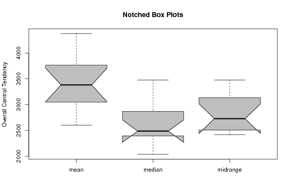
| Title produced by software | Mean Plot | |||||||||||||||||||||||||||||
| Date of computation | Fri, 16 Dec 2016 21:02:14 +0100 | |||||||||||||||||||||||||||||
| Cite this page as follows | Statistical Computations at FreeStatistics.org, Office for Research Development and Education, URL https://freestatistics.org/blog/index.php?v=date/2016/Dec/16/t14819185873n0708nzlobuh78.htm/, Retrieved Thu, 02 May 2024 20:17:07 +0000 | |||||||||||||||||||||||||||||
| Statistical Computations at FreeStatistics.org, Office for Research Development and Education, URL https://freestatistics.org/blog/index.php?pk=300522, Retrieved Thu, 02 May 2024 20:17:07 +0000 | ||||||||||||||||||||||||||||||
| QR Codes: | ||||||||||||||||||||||||||||||
|
| ||||||||||||||||||||||||||||||
| Original text written by user: | ||||||||||||||||||||||||||||||
| IsPrivate? | No (this computation is public) | |||||||||||||||||||||||||||||
| User-defined keywords | ||||||||||||||||||||||||||||||
| Estimated Impact | 57 | |||||||||||||||||||||||||||||
Tree of Dependent Computations | ||||||||||||||||||||||||||||||
| Family? (F = Feedback message, R = changed R code, M = changed R Module, P = changed Parameters, D = changed Data) | ||||||||||||||||||||||||||||||
| - [Mean Plot] [] [2016-12-16 20:02:14] [85f5800284aab30c091766186b093bb4] [Current] | ||||||||||||||||||||||||||||||
| Feedback Forum | ||||||||||||||||||||||||||||||
Post a new message | ||||||||||||||||||||||||||||||
Dataset | ||||||||||||||||||||||||||||||
| Dataseries X: | ||||||||||||||||||||||||||||||
1819,6 1312,4 2584 1479,6 1742 2639,2 1706 1408 1951,6 1690,4 2288,4 2912 1460,8 1009,6 2410 1603,2 2115,2 2330 1690 1358 1806,8 1973,6 1402 1857,6 1974,4 1438 1923,2 1996,8 2238,8 2540,4 1704,4 1856 2214,8 1948 1802 1431,6 2857,6 1784 2770,8 2313,6 3707,6 4322,4 3297,6 2223,6 2136,4 2459,2 1650,4 2921,2 1979,6 1403,2 2374 2876,4 2500 3888 1508,8 1011,2 1590,8 2076,4 3736 2125,6 982,8 2034,8 2260 1726 2270,4 1951,6 2104,4 2972,8 2834,4 4227,6 3392,4 3069,2 3138,8 3570 4800,4 4769,2 5124,8 3476,8 2866,8 2549,2 2728 2448,8 3286,8 2830 3251,2 4188,8 2747,6 2269,2 2493,2 2147,6 2689,2 3557,2 2840 3979,6 2683,2 2852 3012,8 2950,8 3065,2 3942,4 4272 4564 5222,8 5164,4 3883,6 4103,2 5244 8071,6 5441,6 7496 10100,4 9616 5645,6 10490 5582 7579,2 4023,6 8146,4 8534,4 10113,6 8504,4 9782,4 13110 8192,8 8708,8 9528,8 | ||||||||||||||||||||||||||||||
Tables (Output of Computation) | ||||||||||||||||||||||||||||||
| ||||||||||||||||||||||||||||||
Figures (Output of Computation) | ||||||||||||||||||||||||||||||
Input Parameters & R Code | ||||||||||||||||||||||||||||||
| Parameters (Session): | ||||||||||||||||||||||||||||||
| par1 = 12 ; | ||||||||||||||||||||||||||||||
| Parameters (R input): | ||||||||||||||||||||||||||||||
| par1 = 12 ; | ||||||||||||||||||||||||||||||
| R code (references can be found in the software module): | ||||||||||||||||||||||||||||||
par1 <- as.numeric(par1) | ||||||||||||||||||||||||||||||