Free Statistics
of Irreproducible Research!
Description of Statistical Computation | |||||||||||||||||||||
|---|---|---|---|---|---|---|---|---|---|---|---|---|---|---|---|---|---|---|---|---|---|
| Author's title | |||||||||||||||||||||
| Author | *Unverified author* | ||||||||||||||||||||
| R Software Module | rwasp_meanplot.wasp | ||||||||||||||||||||
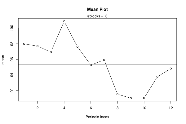
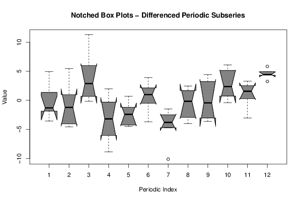
| Title produced by software | Mean Plot | ||||||||||||||||||||
| Date of computation | Sat, 17 Dec 2016 10:20:57 +0000 | ||||||||||||||||||||
| Cite this page as follows | Statistical Computations at FreeStatistics.org, Office for Research Development and Education, URL https://freestatistics.org/blog/index.php?v=date/2016/Dec/17/t1481970110w9jv5p3wq1u8pas.htm/, Retrieved Thu, 02 May 2024 02:35:18 +0200 | ||||||||||||||||||||
| Statistical Computations at FreeStatistics.org, Office for Research Development and Education, URL https://freestatistics.org/blog/index.php?pk=, Retrieved Thu, 02 May 2024 02:35:18 +0200 | |||||||||||||||||||||
| QR Codes: | |||||||||||||||||||||
|
| |||||||||||||||||||||
| Original text written by user: | |||||||||||||||||||||
| IsPrivate? | No (this computation is public) | ||||||||||||||||||||
| User-defined keywords | |||||||||||||||||||||
| Estimated Impact | 0 | ||||||||||||||||||||
Tree of Dependent Computations | |||||||||||||||||||||
Dataset | |||||||||||||||||||||
| Dataseries X: | |||||||||||||||||||||
95,31 93,47 98,92 101,21 95,19 90,95 93,09 90,16 91,86 88,82 91,58 94,9 99,85 98,03 93,46 94,15 93,47 88,98 89,26 84,62 82,7 84,37 89,52 89,82 93,08 98,02 97,49 97,35 99,33 96,92 96,42 93,94 89,95 94,38 95,13 96,01 100,37 99,57 100,53 106,51 106,22 106,93 103,24 98,54 95,6 91,97 93,99 96,53 102,37 98,81 96,88 100,4 91,54 90,36 94,28 84,17 86,65 84,09 90,2 92,47 96,92 98,3 94,27 105,58 99,89 97,46 99,21 97,72 99,31 102,57 102,16 99,12 | |||||||||||||||||||||
Tables (Output of Computation) | |||||||||||||||||||||
| |||||||||||||||||||||
Figures (Output of Computation) | |||||||||||||||||||||
Input Parameters & R Code | |||||||||||||||||||||
| Parameters (Session): | |||||||||||||||||||||
| par1 = 12 ; | |||||||||||||||||||||
| Parameters (R input): | |||||||||||||||||||||
| par1 = 12 ; | |||||||||||||||||||||
| R code (references can be found in the software module): | |||||||||||||||||||||
par1 <- as.numeric(par1) | |||||||||||||||||||||