Free Statistics

of Irreproducible Research!

Author's title

Author*The author of this computation has been verified*
R Software Modulerwasp_decomposeloess.wasp
Title produced by softwareDecomposition by Loess
Date of computationTue, 20 Dec 2016 10:49:25 +0100
Cite this page as followsStatistical Computations at FreeStatistics.org, Office for Research Development and Education, URL https://freestatistics.org/blog/index.php?v=date/2016/Dec/20/t1482227574jwv8ku3kf00b6nd.htm/, Retrieved Sun, 28 Apr 2024 17:28:14 +0000
Statistical Computations at FreeStatistics.org, Office for Research Development and Education, URL https://freestatistics.org/blog/index.php?pk=301560, Retrieved Sun, 28 Apr 2024 17:28:14 +0000
QR Codes:

Original text written by user:
IsPrivate?No (this computation is public)
User-defined keywords
Estimated Impact96
Family? (F = Feedback message, R = changed R code, M = changed R Module, P = changed Parameters, D = changed Data)
-       [Decomposition by Loess] [] [2016-12-20 09:49:25] [b2e25925e4919b0d6985405fcb461c0d] [Current]
Feedback Forum

Post a new message
Dataseries X:
4400
4400
5400
7300
7200
7100
7000
10000
10100
9400
8500
8300
9200
10400
11700
12200
10400
10400
9800
9200


Summary of computational transaction
Raw Input view raw input (R code)
Raw Outputview raw output of R engine
Computing time1 seconds
R ServerBig Analytics Cloud Computing Center

\begin{tabular}{lllllllll}
\hline
Summary of computational transaction \tabularnewline
Raw Input view raw input (R code)  \tabularnewline
Raw Outputview raw output of R engine  \tabularnewline
Computing time1 seconds \tabularnewline
R ServerBig Analytics Cloud Computing Center \tabularnewline
\hline
\end{tabular}
%Source: https://freestatistics.org/blog/index.php?pk=301560&T=0

[TABLE]
[ROW]
Summary of computational transaction[/C][/ROW] [ROW]Raw Input[/C] view raw input (R code) [/C][/ROW] [ROW]Raw Output[/C]view raw output of R engine [/C][/ROW] [ROW]Computing time[/C]1 seconds[/C][/ROW] [ROW]R Server[/C]Big Analytics Cloud Computing Center[/C][/ROW] [/TABLE] Source: https://freestatistics.org/blog/index.php?pk=301560&T=0

Globally Unique Identifier (entire table): ba.freestatistics.org/blog/index.php?pk=301560&T=0

As an alternative you can also use a QR Code:  

The GUIDs for individual cells are displayed in the table below:

Summary of computational transaction
Raw Input view raw input (R code)
Raw Outputview raw output of R engine
Computing time1 seconds
R ServerBig Analytics Cloud Computing Center


Seasonal Decomposition by Loess - Parameters
ComponentWindowDegreeJump
Seasonal201021
Trend1512
Low-pass911

\begin{tabular}{lllllllll}
\hline
Seasonal Decomposition by Loess - Parameters \tabularnewline
Component & Window & Degree & Jump \tabularnewline
Seasonal & 201 & 0 & 21 \tabularnewline
Trend & 15 & 1 & 2 \tabularnewline
Low-pass & 9 & 1 & 1 \tabularnewline
\hline
\end{tabular}
%Source: https://freestatistics.org/blog/index.php?pk=301560&T=1

[TABLE]
[ROW][C]Seasonal Decomposition by Loess - Parameters[/C][/ROW]
[ROW][C]Component[/C][C]Window[/C][C]Degree[/C][C]Jump[/C][/ROW]
[ROW][C]Seasonal[/C][C]201[/C][C]0[/C][C]21[/C][/ROW]
[ROW][C]Trend[/C][C]15[/C][C]1[/C][C]2[/C][/ROW]
[ROW][C]Low-pass[/C][C]9[/C][C]1[/C][C]1[/C][/ROW]
[/TABLE]
Source: https://freestatistics.org/blog/index.php?pk=301560&T=1

Globally Unique Identifier (entire table): ba.freestatistics.org/blog/index.php?pk=301560&T=1

As an alternative you can also use a QR Code:  

The GUIDs for individual cells are displayed in the table below:

Seasonal Decomposition by Loess - Parameters
ComponentWindowDegreeJump
Seasonal201021
Trend1512
Low-pass911


Seasonal Decomposition by Loess - Time Series Components
tObservedFittedSeasonalTrendRemainder
144004013.56886974221-461.2494349760365247.68056523382-386.431130257788
244004343.6318056555-1226.406970042985682.77516438747-56.3681943444972
354005907.06416131648-1224.93392485766117.86976354112507.064161316481
473008197.46926342228-158.8377703024316561.36850688016897.469263422276
572007210.8100432832184.3227064976147004.8672502191910.8100432831961
671006182.67834200363572.530890706137444.79076729024-917.321657996368
770005563.29196576204551.9937498766787884.71428436128-1436.70803423796
81000010791.6618623396951.383505565258256.95463209512791.66186233963
91010010759.6078568047811.1971633663368629.19497982896659.607856804707
10940010234.8839341062-461.2494349760369026.36550086981834.88393410623
1185008802.87094813232-1226.406970042989423.53602191066302.87094813232
1283008120.50931729304-1224.93392485769704.42460756456-179.490682706959
1392008573.52457708396-158.8377703024319985.31319321847-626.475422916037
141040010572.6807966122184.32270649761410042.9964968902172.680796612165
151170012726.7893087319572.5308907061310100.6798005621026.7893087319
161220013675.7741325868551.99374987667810172.23211753651475.77413258683
17104009604.83205992374951.3835055652510243.784434511-795.167940076259
18104009686.42658477865811.19716336633610302.376251855-713.57341522135
1998009700.28136577702-461.24943497603610360.968069199-99.7186342229797
2092009220.57131531841-1226.4069700429810405.835654724620.5713153184133

\begin{tabular}{lllllllll}
\hline
Seasonal Decomposition by Loess - Time Series Components \tabularnewline
t & Observed & Fitted & Seasonal & Trend & Remainder \tabularnewline
1 & 4400 & 4013.56886974221 & -461.249434976036 & 5247.68056523382 & -386.431130257788 \tabularnewline
2 & 4400 & 4343.6318056555 & -1226.40697004298 & 5682.77516438747 & -56.3681943444972 \tabularnewline
3 & 5400 & 5907.06416131648 & -1224.9339248576 & 6117.86976354112 & 507.064161316481 \tabularnewline
4 & 7300 & 8197.46926342228 & -158.837770302431 & 6561.36850688016 & 897.469263422276 \tabularnewline
5 & 7200 & 7210.8100432832 & 184.322706497614 & 7004.86725021919 & 10.8100432831961 \tabularnewline
6 & 7100 & 6182.67834200363 & 572.53089070613 & 7444.79076729024 & -917.321657996368 \tabularnewline
7 & 7000 & 5563.29196576204 & 551.993749876678 & 7884.71428436128 & -1436.70803423796 \tabularnewline
8 & 10000 & 10791.6618623396 & 951.38350556525 & 8256.95463209512 & 791.66186233963 \tabularnewline
9 & 10100 & 10759.6078568047 & 811.197163366336 & 8629.19497982896 & 659.607856804707 \tabularnewline
10 & 9400 & 10234.8839341062 & -461.249434976036 & 9026.36550086981 & 834.88393410623 \tabularnewline
11 & 8500 & 8802.87094813232 & -1226.40697004298 & 9423.53602191066 & 302.87094813232 \tabularnewline
12 & 8300 & 8120.50931729304 & -1224.9339248576 & 9704.42460756456 & -179.490682706959 \tabularnewline
13 & 9200 & 8573.52457708396 & -158.837770302431 & 9985.31319321847 & -626.475422916037 \tabularnewline
14 & 10400 & 10572.6807966122 & 184.322706497614 & 10042.9964968902 & 172.680796612165 \tabularnewline
15 & 11700 & 12726.7893087319 & 572.53089070613 & 10100.679800562 & 1026.7893087319 \tabularnewline
16 & 12200 & 13675.7741325868 & 551.993749876678 & 10172.2321175365 & 1475.77413258683 \tabularnewline
17 & 10400 & 9604.83205992374 & 951.38350556525 & 10243.784434511 & -795.167940076259 \tabularnewline
18 & 10400 & 9686.42658477865 & 811.197163366336 & 10302.376251855 & -713.57341522135 \tabularnewline
19 & 9800 & 9700.28136577702 & -461.249434976036 & 10360.968069199 & -99.7186342229797 \tabularnewline
20 & 9200 & 9220.57131531841 & -1226.40697004298 & 10405.8356547246 & 20.5713153184133 \tabularnewline
\hline
\end{tabular}
%Source: https://freestatistics.org/blog/index.php?pk=301560&T=2

[TABLE]
[ROW][C]Seasonal Decomposition by Loess - Time Series Components[/C][/ROW]
[ROW][C]t[/C][C]Observed[/C][C]Fitted[/C][C]Seasonal[/C][C]Trend[/C][C]Remainder[/C][/ROW]
[ROW][C]1[/C][C]4400[/C][C]4013.56886974221[/C][C]-461.249434976036[/C][C]5247.68056523382[/C][C]-386.431130257788[/C][/ROW]
[ROW][C]2[/C][C]4400[/C][C]4343.6318056555[/C][C]-1226.40697004298[/C][C]5682.77516438747[/C][C]-56.3681943444972[/C][/ROW]
[ROW][C]3[/C][C]5400[/C][C]5907.06416131648[/C][C]-1224.9339248576[/C][C]6117.86976354112[/C][C]507.064161316481[/C][/ROW]
[ROW][C]4[/C][C]7300[/C][C]8197.46926342228[/C][C]-158.837770302431[/C][C]6561.36850688016[/C][C]897.469263422276[/C][/ROW]
[ROW][C]5[/C][C]7200[/C][C]7210.8100432832[/C][C]184.322706497614[/C][C]7004.86725021919[/C][C]10.8100432831961[/C][/ROW]
[ROW][C]6[/C][C]7100[/C][C]6182.67834200363[/C][C]572.53089070613[/C][C]7444.79076729024[/C][C]-917.321657996368[/C][/ROW]
[ROW][C]7[/C][C]7000[/C][C]5563.29196576204[/C][C]551.993749876678[/C][C]7884.71428436128[/C][C]-1436.70803423796[/C][/ROW]
[ROW][C]8[/C][C]10000[/C][C]10791.6618623396[/C][C]951.38350556525[/C][C]8256.95463209512[/C][C]791.66186233963[/C][/ROW]
[ROW][C]9[/C][C]10100[/C][C]10759.6078568047[/C][C]811.197163366336[/C][C]8629.19497982896[/C][C]659.607856804707[/C][/ROW]
[ROW][C]10[/C][C]9400[/C][C]10234.8839341062[/C][C]-461.249434976036[/C][C]9026.36550086981[/C][C]834.88393410623[/C][/ROW]
[ROW][C]11[/C][C]8500[/C][C]8802.87094813232[/C][C]-1226.40697004298[/C][C]9423.53602191066[/C][C]302.87094813232[/C][/ROW]
[ROW][C]12[/C][C]8300[/C][C]8120.50931729304[/C][C]-1224.9339248576[/C][C]9704.42460756456[/C][C]-179.490682706959[/C][/ROW]
[ROW][C]13[/C][C]9200[/C][C]8573.52457708396[/C][C]-158.837770302431[/C][C]9985.31319321847[/C][C]-626.475422916037[/C][/ROW]
[ROW][C]14[/C][C]10400[/C][C]10572.6807966122[/C][C]184.322706497614[/C][C]10042.9964968902[/C][C]172.680796612165[/C][/ROW]
[ROW][C]15[/C][C]11700[/C][C]12726.7893087319[/C][C]572.53089070613[/C][C]10100.679800562[/C][C]1026.7893087319[/C][/ROW]
[ROW][C]16[/C][C]12200[/C][C]13675.7741325868[/C][C]551.993749876678[/C][C]10172.2321175365[/C][C]1475.77413258683[/C][/ROW]
[ROW][C]17[/C][C]10400[/C][C]9604.83205992374[/C][C]951.38350556525[/C][C]10243.784434511[/C][C]-795.167940076259[/C][/ROW]
[ROW][C]18[/C][C]10400[/C][C]9686.42658477865[/C][C]811.197163366336[/C][C]10302.376251855[/C][C]-713.57341522135[/C][/ROW]
[ROW][C]19[/C][C]9800[/C][C]9700.28136577702[/C][C]-461.249434976036[/C][C]10360.968069199[/C][C]-99.7186342229797[/C][/ROW]
[ROW][C]20[/C][C]9200[/C][C]9220.57131531841[/C][C]-1226.40697004298[/C][C]10405.8356547246[/C][C]20.5713153184133[/C][/ROW]
[/TABLE]
Source: https://freestatistics.org/blog/index.php?pk=301560&T=2

Globally Unique Identifier (entire table): ba.freestatistics.org/blog/index.php?pk=301560&T=2

As an alternative you can also use a QR Code:  

The GUIDs for individual cells are displayed in the table below:

Seasonal Decomposition by Loess - Time Series Components
tObservedFittedSeasonalTrendRemainder
144004013.56886974221-461.2494349760365247.68056523382-386.431130257788
244004343.6318056555-1226.406970042985682.77516438747-56.3681943444972
354005907.06416131648-1224.93392485766117.86976354112507.064161316481
473008197.46926342228-158.8377703024316561.36850688016897.469263422276
572007210.8100432832184.3227064976147004.8672502191910.8100432831961
671006182.67834200363572.530890706137444.79076729024-917.321657996368
770005563.29196576204551.9937498766787884.71428436128-1436.70803423796
81000010791.6618623396951.383505565258256.95463209512791.66186233963
91010010759.6078568047811.1971633663368629.19497982896659.607856804707
10940010234.8839341062-461.2494349760369026.36550086981834.88393410623
1185008802.87094813232-1226.406970042989423.53602191066302.87094813232
1283008120.50931729304-1224.93392485769704.42460756456-179.490682706959
1392008573.52457708396-158.8377703024319985.31319321847-626.475422916037
141040010572.6807966122184.32270649761410042.9964968902172.680796612165
151170012726.7893087319572.5308907061310100.6798005621026.7893087319
161220013675.7741325868551.99374987667810172.23211753651475.77413258683
17104009604.83205992374951.3835055652510243.784434511-795.167940076259
18104009686.42658477865811.19716336633610302.376251855-713.57341522135
1998009700.28136577702-461.24943497603610360.968069199-99.7186342229797
2092009220.57131531841-1226.4069700429810405.835654724620.5713153184133


Parameters (Session):
par1 = 60 ; par2 = 1 ; par3 = 1 ; par4 = 1 ; par5 = 12 ; par6 = White Noise ; par7 = 0.95 ;
Parameters (R input):
par1 = 9 ; par2 = periodic ; par3 = 0 ; par4 = ; par5 = 1 ; par6 = ; par7 = 1 ; par8 = FALSE ;
R code (references can be found in the software module):
par8 <- 'FALSE'
par7 <- '1'
par6 <- ''
par5 <- '1'
par4 <- ''
par3 <- '0'
par2 <- 'periodic'
par1 <- '6'
par1 <- as.numeric(par1) #seasonal period
if (par2 != 'periodic') par2 <- as.numeric(par2) #s.window
par3 <- as.numeric(par3) #s.degree
if (par4 == '') par4 <- NULL else par4 <- as.numeric(par4)#t.window
par5 <- as.numeric(par5)#t.degree
if (par6 != '') par6 <- as.numeric(par6)#l.window
par7 <- as.numeric(par7)#l.degree
if (par8 == 'FALSE') par8 <- FALSE else par9 <- TRUE #robust
nx <- length(x)
x <- ts(x,frequency=par1)
if (par6 != '') {
m <- stl(x,s.window=par2, s.degree=par3, t.window=par4, t.degre=par5, l.window=par6, l.degree=par7, robust=par8)
} else {
m <- stl(x,s.window=par2, s.degree=par3, t.window=par4, t.degre=par5, l.degree=par7, robust=par8)
}
m$time.series
m$win
m$deg
m$jump
m$inner
m$outer
bitmap(file='test1.png')
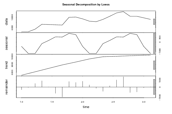
plot(m,main=main)
dev.off()
mylagmax <- nx/2
bitmap(file='test2.png')
op <- par(mfrow = c(2,2))
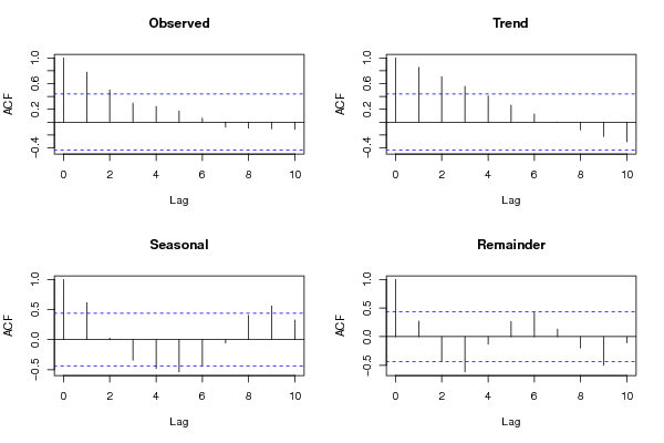
acf(as.numeric(x),lag.max = mylagmax,main='Observed')
acf(as.numeric(m$time.series[,'trend']),na.action=na.pass,lag.max = mylagmax,main='Trend')
acf(as.numeric(m$time.series[,'seasonal']),na.action=na.pass,lag.max = mylagmax,main='Seasonal')
acf(as.numeric(m$time.series[,'remainder']),na.action=na.pass,lag.max = mylagmax,main='Remainder')
par(op)
dev.off()
bitmap(file='test3.png')
op <- par(mfrow = c(2,2))
spectrum(as.numeric(x),main='Observed')
spectrum(as.numeric(m$time.series[!is.na(m$time.series[,'trend']),'trend']),main='Trend')
spectrum(as.numeric(m$time.series[!is.na(m$time.series[,'seasonal']),'seasonal']),main='Seasonal')
spectrum(as.numeric(m$time.series[!is.na(m$time.series[,'remainder']),'remainder']),main='Remainder')
par(op)
dev.off()
bitmap(file='test4.png')
op <- par(mfrow = c(2,2))
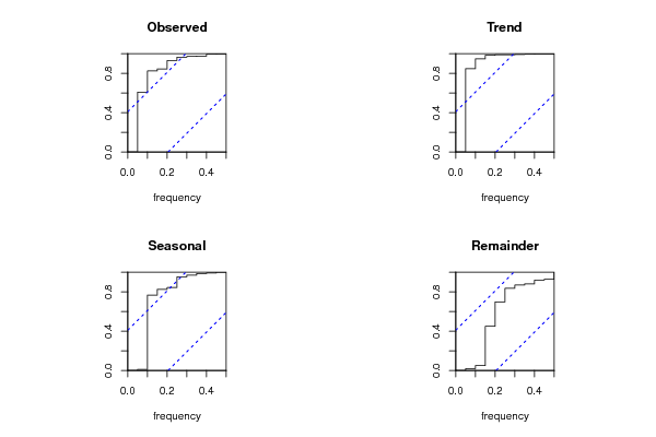
cpgram(as.numeric(x),main='Observed')
cpgram(as.numeric(m$time.series[!is.na(m$time.series[,'trend']),'trend']),main='Trend')
cpgram(as.numeric(m$time.series[!is.na(m$time.series[,'seasonal']),'seasonal']),main='Seasonal')
cpgram(as.numeric(m$time.series[!is.na(m$time.series[,'remainder']),'remainder']),main='Remainder')
par(op)
dev.off()
load(file='createtable')
a<-table.start()
a<-table.row.start(a)
a<-table.element(a,'Seasonal Decomposition by Loess - Parameters',4,TRUE)
a<-table.row.end(a)
a<-table.row.start(a)
a<-table.element(a,'Component',header=TRUE)
a<-table.element(a,'Window',header=TRUE)
a<-table.element(a,'Degree',header=TRUE)
a<-table.element(a,'Jump',header=TRUE)
a<-table.row.end(a)
a<-table.row.start(a)
a<-table.element(a,'Seasonal',header=TRUE)
a<-table.element(a,m$win['s'])
a<-table.element(a,m$deg['s'])
a<-table.element(a,m$jump['s'])
a<-table.row.end(a)
a<-table.row.start(a)
a<-table.element(a,'Trend',header=TRUE)
a<-table.element(a,m$win['t'])
a<-table.element(a,m$deg['t'])
a<-table.element(a,m$jump['t'])
a<-table.row.end(a)
a<-table.row.start(a)
a<-table.element(a,'Low-pass',header=TRUE)
a<-table.element(a,m$win['l'])
a<-table.element(a,m$deg['l'])
a<-table.element(a,m$jump['l'])
a<-table.row.end(a)
a<-table.end(a)
table.save(a,file='mytable.tab')
a<-table.start()
a<-table.row.start(a)
a<-table.element(a,'Seasonal Decomposition by Loess - Time Series Components',6,TRUE)
a<-table.row.end(a)
a<-table.row.start(a)
a<-table.element(a,'t',header=TRUE)
a<-table.element(a,'Observed',header=TRUE)
a<-table.element(a,'Fitted',header=TRUE)
a<-table.element(a,'Seasonal',header=TRUE)
a<-table.element(a,'Trend',header=TRUE)
a<-table.element(a,'Remainder',header=TRUE)
a<-table.row.end(a)
for (i in 1:nx) {
a<-table.row.start(a)
a<-table.element(a,i,header=TRUE)
a<-table.element(a,x[i])
a<-table.element(a,x[i]+m$time.series[i,'remainder'])
a<-table.element(a,m$time.series[i,'seasonal'])
a<-table.element(a,m$time.series[i,'trend'])
a<-table.element(a,m$time.series[i,'remainder'])
a<-table.row.end(a)
}
a<-table.end(a)
table.save(a,file='mytable1.tab')