Repository of Reproducible Computations

Free Statistics

of Irreproducible Research!

Author's title

Author

*The author of this computation has been verified*

R Software Module

rwasp_fitdistrnorm.wasp

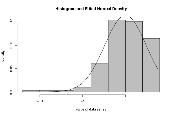
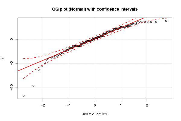
Title produced by software

ML Fitting and QQ Plot- Normal Distribution

Date of computation

Wed, 21 Dec 2016 21:29:12 +0100

Cite this page as follows

Statistical Computations at FreeStatistics.org, Office for Research Development and Education, URL https://freestatistics.org/blog/index.php?v=date/2016/Dec/21/t1482352223rrptdj5kj6zaxmt.htm/, Retrieved Mon, 06 May 2024 14:01:36 +0000

Statistical Computations at FreeStatistics.org, Office for Research Development and Education, URL https://freestatistics.org/blog/index.php?pk=302493, Retrieved Mon, 06 May 2024 14:01:36 +0000

QR Codes:

Paste this QR Code to cite your computation.

Original text written by user:

IsPrivate?

No (this computation is public)

User-defined keywords

Estimated Impact

Family? (F = Feedback message, R = changed R code, M = changed R Module, P = changed Parameters, D = changed Data)

-       [ML Fitting and QQ Plot- Normal Distribution] [QQ plot] [2016-12-21 20:29:12] [6f830dc7e8de22be3233942ffbe3aaba] [Current]

Feedback Forum

Post a new message

Dataseries X:

Download CSV

Histogram

Boxplots

-1.893
2.514
0.141
0.624
-1.376
3.18
-1.82
2.216
-1.784
-1.894
2.106
-0.376
3.624
1.699
-1.376
-2.894
3.624
-0.2662
-0.7844
-0.4859
-6.376
2.514
2.624
-0.7844
-1.6
1.624
0.624
2.216
0.2156
-1.858
2.29
3.514
-11.78
2.773
-0.8942
-1.376
-0.1915
1.844
-0.8942
-1.376
0.1058
-1.893
3.216
2.624
-9.674
-3.784
-0.376
0.1422
1.106
1.031
-0.5605
1.327
2.734
-0.1563
2.624
-3.56
-0.376
-3.376
-4.894
0.5141
0.5494
0.5141
-0.376
-0.2268
-2.894
-0.2662
-3.156
-0.4859
-2.376
3.624
-3.968
-3.192
1.44
-2.376
2.18
1.734
-2.156
1.106
2.216
-0.5635
-2.784
0.5141
2.216
-3.969
2.216
1.106
3.624
-1.486
-0.6692
-1.376
3.141
-1.784
2.141
1.624
1.624
-1.451
3.106
0.5141
1.216
2.624
3.844
-3.376
0.2156
-1.376
-0.7844
1.624
1.624
-2.376
-0.9677
-4.376
1.217
-2.894
1.624
0.5141
0.2156
3.514
-0.2662
-2.376
-1.266
1.624
3.624
0.2156
0.624
0.5141
0.2156
-1.376
0.624
2.327
0.624
3.549
-1.192
0.3267
-1.376
1.216
-1.376
1.031
3.141
2.808
-2.266
-0.376
-0.8578
0.141
1.844
3.031
0.6986
1.624
-0.7832
-0.376
-5.486
-1.376
2.252
0.624
-0.8942
-3.968
2.624
1.106
-1.376
0.03117
2.734
1.624
2.624
-0.1915
-0.376
0.03232
-2.266

Summary of computational transaction
Raw Input	view raw input (R code)
Raw Output	view raw output of R engine
Computing time	4 seconds
R Server	Big Analytics Cloud Computing Center

\begin{tabular}{lllllllll}
\hline
Summary of computational transaction \tabularnewline
Raw Input view raw input (R code)  \tabularnewline
Raw Outputview raw output of R engine  \tabularnewline
Computing time4 seconds \tabularnewline
R ServerBig Analytics Cloud Computing Center \tabularnewline
\hline
\end{tabular}
%Source: https://freestatistics.org/blog/index.php?pk=302493&T=0

[TABLE]
[ROW]

Summary of computational transaction[/C][/ROW] [ROW]

Raw Input[/C]

view raw input (R code) [/C][/ROW] [ROW]

Raw Output[/C]

view raw output of R engine [/C][/ROW] [ROW]

Computing time[/C]

4 seconds[/C][/ROW] [ROW]

R Server[/C]

Big Analytics Cloud Computing Center[/C][/ROW] [/TABLE] Source: https://freestatistics.org/blog/index.php?pk=302493&T=0

Globally Unique Identifier (entire table): ba.freestatistics.org/blog/index.php?pk=302493&T=0

As an alternative you can also use a QR Code:

The GUIDs for individual cells are displayed in the table below:

Summary of computational transaction
Raw Input	view raw input (R code)
Raw Output	view raw output of R engine
Computing time	4 seconds
R Server	Big Analytics Cloud Computing Center

Parameter	Estimated Value	Standard Deviation
mean	6.41818181818458e-05	0.188750275227852
standard deviation	2.42454118458882	0.133466599564442

\begin{tabular}{lllllllll}
\hline
Parameter & Estimated Value & Standard Deviation \tabularnewline
mean & 6.41818181818458e-05 & 0.188750275227852 \tabularnewline
standard deviation & 2.42454118458882 & 0.133466599564442 \tabularnewline
\hline
\end{tabular}
%Source: https://freestatistics.org/blog/index.php?pk=302493&T=1

[TABLE]
[ROW][C]Parameter[/C][C]Estimated Value[/C][C]Standard Deviation[/C][/ROW]
[ROW][C]mean[/C][C]6.41818181818458e-05[/C][C]0.188750275227852[/C][/ROW]
[ROW][C]standard deviation[/C][C]2.42454118458882[/C][C]0.133466599564442[/C][/ROW]
[/TABLE]
Source: https://freestatistics.org/blog/index.php?pk=302493&T=1

Globally Unique Identifier (entire table): ba.freestatistics.org/blog/index.php?pk=302493&T=1

As an alternative you can also use a QR Code:

The GUIDs for individual cells are displayed in the table below:

Parameter	Estimated Value	Standard Deviation
mean	6.41818181818458e-05	0.188750275227852
standard deviation	2.42454118458882	0.133466599564442

Figure 1

PNG link

Postscript link

PDF link

Figure 2

PNG link

Postscript link

PDF link

Parameters (Session):

par1 = 8 ; par2 = 0 ;

Parameters (R input):

par1 = 8 ; par2 = 0 ;

R code (references can be found in the software module):

library(MASS)
library(car)
par1 <- as.numeric(par1)
if (par2 == '0') par2 = 'Sturges' else par2 <- as.numeric(par2)
x <- as.ts(x) #otherwise the fitdistr function does not work properly
r <- fitdistr(x,'normal')
print(r)
bitmap(file='test1.png')
myhist<-hist(x,col=par1,breaks=par2,main=main,ylab=ylab,xlab=xlab,freq=F)
curve(1/(r$estimate[2]*sqrt(2*pi))*exp(-1/2*((x-r$estimate[1])/r$estimate[2])^2),min(x),max(x),add=T)
dev.off()
bitmap(file='test3.png')
qqPlot(x,dist='norm',main='QQ plot (Normal) with confidence intervals')
grid()
dev.off()
load(file='createtable')
a<-table.start()
a<-table.row.start(a)
a<-table.element(a,'Parameter',1,TRUE)
a<-table.element(a,'Estimated Value',1,TRUE)
a<-table.element(a,'Standard Deviation',1,TRUE)
a<-table.row.end(a)
a<-table.row.start(a)
a<-table.element(a,'mean',header=TRUE)
a<-table.element(a,r$estimate[1])
a<-table.element(a,r$sd[1])
a<-table.row.end(a)
a<-table.row.start(a)
a<-table.element(a,'standard deviation',header=TRUE)
a<-table.element(a,r$estimate[2])
a<-table.element(a,r$sd[2])
a<-table.row.end(a)
a<-table.end(a)
table.save(a,file='mytable.tab')

Free Statistics

Description of Statistical Computation

Tree of Dependent Computations

Dataset

Tables (Output of Computation)

Figures (Output of Computation)

Input Parameters & R Code