Free Statistics
of Irreproducible Research!
Description of Statistical Computation | |||||||||||||||||||||
|---|---|---|---|---|---|---|---|---|---|---|---|---|---|---|---|---|---|---|---|---|---|
| Author's title | |||||||||||||||||||||
| Author | *Unverified author* | ||||||||||||||||||||
| R Software Module | rwasp_meanplot.wasp | ||||||||||||||||||||
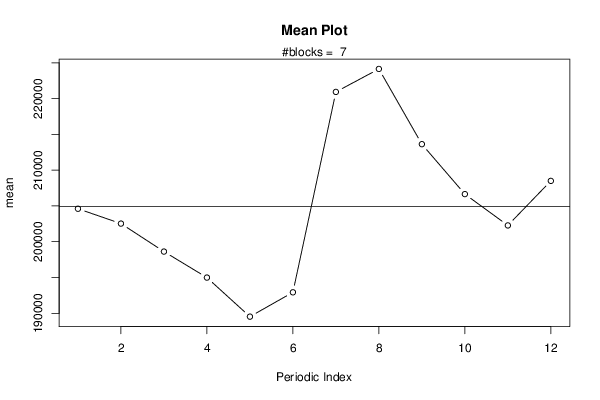
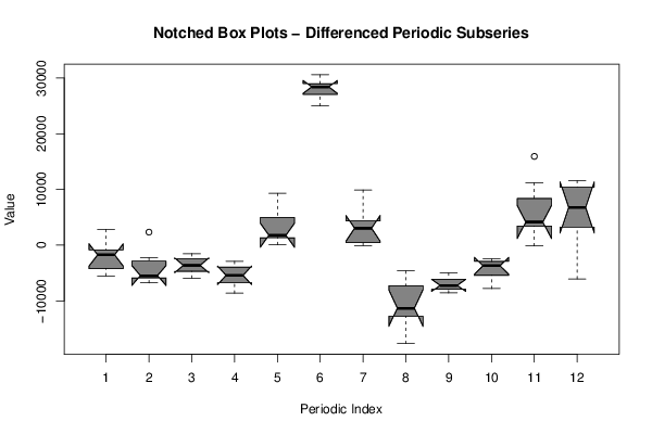
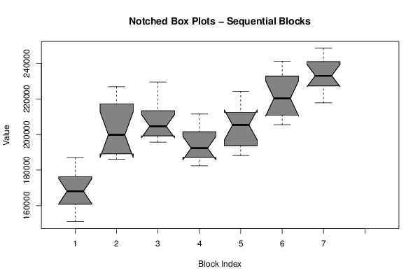
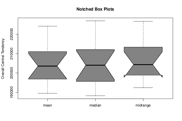
| Title produced by software | Mean Plot | ||||||||||||||||||||
| Date of computation | Fri, 08 Jan 2016 12:15:10 +0000 | ||||||||||||||||||||
| Cite this page as follows | Statistical Computations at FreeStatistics.org, Office for Research Development and Education, URL https://freestatistics.org/blog/index.php?v=date/2016/Jan/08/t145225545586y7n348xf7xxvj.htm/, Retrieved Sun, 28 Apr 2024 07:40:50 +0000 | ||||||||||||||||||||
| Statistical Computations at FreeStatistics.org, Office for Research Development and Education, URL https://freestatistics.org/blog/index.php?pk=287410, Retrieved Sun, 28 Apr 2024 07:40:50 +0000 | |||||||||||||||||||||
| QR Codes: | |||||||||||||||||||||
|
| |||||||||||||||||||||
| Original text written by user: | |||||||||||||||||||||
| IsPrivate? | No (this computation is public) | ||||||||||||||||||||
| User-defined keywords | |||||||||||||||||||||
| Estimated Impact | 141 | ||||||||||||||||||||
Tree of Dependent Computations | |||||||||||||||||||||
| Family? (F = Feedback message, R = changed R code, M = changed R Module, P = changed Parameters, D = changed Data) | |||||||||||||||||||||
| - [Mean Plot] [cijfergegevens-op...] [2015-10-23 08:29:11] [148b14c5dbcad3a1bad7729b47ff94ec] - R D [Mean Plot] [Verbetering opgav...] [2016-01-08 12:15:10] [df110f336183c9d15b985c5fac87d8f5] [Current] | |||||||||||||||||||||
| Feedback Forum | |||||||||||||||||||||
Post a new message | |||||||||||||||||||||
Dataset | |||||||||||||||||||||
| Dataseries X: | |||||||||||||||||||||
169701 164182 161914 159612 151001 158114 186530 187069 174330 169362 166827 178037 186412 189226 191563 188906 186005 195309 223532 226899 214126 206903 204442 220376 214320 212588 205816 202196 195722 198563 229139 229527 211868 203555 195770 199834 203089 198480 192684 187827 182414 182510 211524 211451 200140 191568 186424 191987 203583 201920 195978 191395 188222 189422 214419 224325 216222 210506 207221 210027 215191 215177 211701 210176 205491 206996 235980 241292 236675 229127 225436 229570 239973 236168 230703 224790 217811 219576 245472 248511 242084 235572 229827 229697 | |||||||||||||||||||||
Tables (Output of Computation) | |||||||||||||||||||||
| |||||||||||||||||||||
Figures (Output of Computation) | |||||||||||||||||||||
Input Parameters & R Code | |||||||||||||||||||||
| Parameters (Session): | |||||||||||||||||||||
| par1 = 12 ; | |||||||||||||||||||||
| Parameters (R input): | |||||||||||||||||||||
| par1 = 12 ; | |||||||||||||||||||||
| R code (references can be found in the software module): | |||||||||||||||||||||
par1 <- as.numeric(par1) | |||||||||||||||||||||