Free Statistics
of Irreproducible Research!
Description of Statistical Computation | |||||||||||||||||||||||||||||||||||||||
|---|---|---|---|---|---|---|---|---|---|---|---|---|---|---|---|---|---|---|---|---|---|---|---|---|---|---|---|---|---|---|---|---|---|---|---|---|---|---|---|
| Author's title | |||||||||||||||||||||||||||||||||||||||
| Author | *The author of this computation has been verified* | ||||||||||||||||||||||||||||||||||||||
| R Software Module | rwasp_fitdistrnorm.wasp | ||||||||||||||||||||||||||||||||||||||
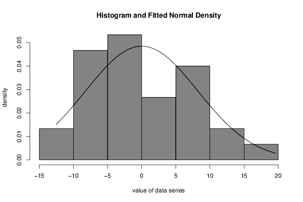
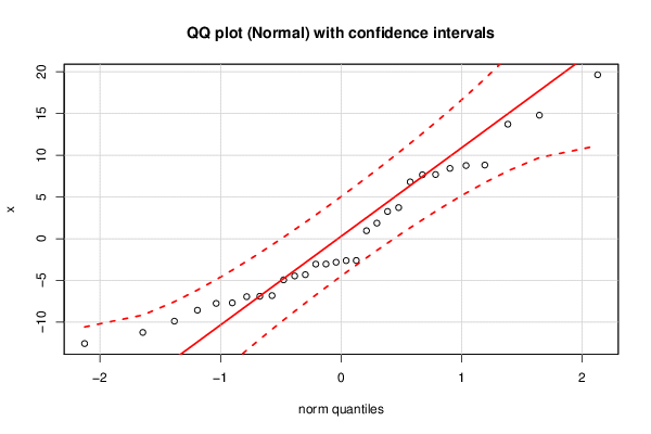
| Title produced by software | ML Fitting and QQ Plot- Normal Distribution | ||||||||||||||||||||||||||||||||||||||
| Date of computation | Thu, 21 Jan 2016 09:05:49 +0000 | ||||||||||||||||||||||||||||||||||||||
| Cite this page as follows | Statistical Computations at FreeStatistics.org, Office for Research Development and Education, URL https://freestatistics.org/blog/index.php?v=date/2016/Jan/21/t1453367155qusgwtjrd98orn0.htm/, Retrieved Sun, 28 Apr 2024 22:21:59 +0000 | ||||||||||||||||||||||||||||||||||||||
| Statistical Computations at FreeStatistics.org, Office for Research Development and Education, URL https://freestatistics.org/blog/index.php?pk=289821, Retrieved Sun, 28 Apr 2024 22:21:59 +0000 | |||||||||||||||||||||||||||||||||||||||
| QR Codes: | |||||||||||||||||||||||||||||||||||||||
|
| |||||||||||||||||||||||||||||||||||||||
| Original text written by user: | |||||||||||||||||||||||||||||||||||||||
| IsPrivate? | No (this computation is public) | ||||||||||||||||||||||||||||||||||||||
| User-defined keywords | |||||||||||||||||||||||||||||||||||||||
| Estimated Impact | 132 | ||||||||||||||||||||||||||||||||||||||
Tree of Dependent Computations | |||||||||||||||||||||||||||||||||||||||
| Family? (F = Feedback message, R = changed R code, M = changed R Module, P = changed Parameters, D = changed Data) | |||||||||||||||||||||||||||||||||||||||
| - [Survey Scores] [] [2015-09-26 10:29:29] [32b17a345b130fdf5cc88718ed94a974] - RMPD [Mean Plot] [] [2015-10-12 12:45:54] [32b17a345b130fdf5cc88718ed94a974] - RMPD [Testing Mean with unknown Variance - Critical Value] [Gemiddelde waarde...] [2016-01-21 07:34:29] [0c1fa16ee907241ae059273f78b5ef86] - RM D [ML Fitting and QQ Plot- Normal Distribution] [] [2016-01-21 09:05:49] [e1c47852802a108fd71d384bb5b16903] [Current] | |||||||||||||||||||||||||||||||||||||||
| Feedback Forum | |||||||||||||||||||||||||||||||||||||||
Post a new message | |||||||||||||||||||||||||||||||||||||||
Dataset | |||||||||||||||||||||||||||||||||||||||
| Dataseries X: | |||||||||||||||||||||||||||||||||||||||
19.6427 13.7242 14.8027 8.42832 6.80835 8.82499 8.76937 7.69536 7.65933 1.86731 3.72965 3.26542 -7.7517 0.957393 -3.04433 -12.5655 -6.9441 -6.8168 -8.56987 -4.46034 -11.229 -3.03305 -9.87928 -4.30931 -2.82241 -2.62636 -4.92814 -2.61029 -6.89788 -7.6867 | |||||||||||||||||||||||||||||||||||||||
Tables (Output of Computation) | |||||||||||||||||||||||||||||||||||||||
| |||||||||||||||||||||||||||||||||||||||
Figures (Output of Computation) | |||||||||||||||||||||||||||||||||||||||
Input Parameters & R Code | |||||||||||||||||||||||||||||||||||||||
| Parameters (Session): | |||||||||||||||||||||||||||||||||||||||
| par1 = 6 ; par2 = grey ; par3 = FALSE ; par4 = 7-point Likert ; | |||||||||||||||||||||||||||||||||||||||
| Parameters (R input): | |||||||||||||||||||||||||||||||||||||||
| par1 = 8 ; par2 = 0 ; | |||||||||||||||||||||||||||||||||||||||
| R code (references can be found in the software module): | |||||||||||||||||||||||||||||||||||||||
library(MASS) | |||||||||||||||||||||||||||||||||||||||