Free Statistics

of Irreproducible Research!

Author's title

Author*The author of this computation has been verified*
R Software Modulerwasp_arimabackwardselection.wasp
Title produced by softwareARIMA Backward Selection
Date of computationThu, 21 Jan 2016 15:30:00 +0000
Cite this page as followsStatistical Computations at FreeStatistics.org, Office for Research Development and Education, URL https://freestatistics.org/blog/index.php?v=date/2016/Jan/21/t1453390672rbbbocjkm7jo60a.htm/, Retrieved Sun, 28 Apr 2024 21:45:14 +0000
Statistical Computations at FreeStatistics.org, Office for Research Development and Education, URL https://freestatistics.org/blog/index.php?pk=289910, Retrieved Sun, 28 Apr 2024 21:45:14 +0000
QR Codes:

Original text written by user:
IsPrivate?No (this computation is public)
User-defined keywords
Estimated Impact74
Family? (F = Feedback message, R = changed R code, M = changed R Module, P = changed Parameters, D = changed Data)
-       [ARIMA Backward Selection] [] [2016-01-21 15:30:00] [074449c5cdcdb4dafd7dd3585d12ae02] [Current]
Feedback Forum

Post a new message
Dataseries X:
0.0013999990894105
0.0876771622176185
0.253920154859331
-0.0329407507841036
0.00427395855379008
-0.0889668134958849
-0.165281368150775
-0.33220433089751
0.219927126513421
0.236701919529402
0.234525437835356
-0.0304289243382355
0.0953913592916723
0.222671044416315
0.0914666084830592
-0.206034580848975
0.317983507811223
0.209887369047125
0.47505736015715
-0.222062521324981
0.0119408639911758
-0.172481528037084
-0.342720660187122
-0.343867756086308
0.088435724392957
0.207149951929822
0.0343760117343465
-0.301707672057424
-0.0110173444677831
-0.0691482212286872
-0.925838573157798
0.137673245546374
0.0727565374056945
0.201173883123843
0.0856783035058499
-0.109577212438584
-0.260551934204086
0.147885882041203
0.212413648519748
-0.0832851309957541
-0.115216896092894
-0.221533847078893
0.33793754507397
-0.134446101735477
0.164631582429395
0.0888222485881065
0.0469533479921545
0.241738416214495
-0.0752540261587926
-0.0299598595890917
0.225881103587503
0.0412636104361186
0.128108276344458
-0.141250457347375
0.481091241511557
-0.11016711751824
0.191801843198123
-0.066757083135655
0.0394798962983962
-0.0743907512944395
0.0864476825544102
-0.0321810065262648
0.121406171476103
-0.0784677853924106
-0.219288911182277
-0.0373619502368736
0.449190378168538
-0.083495394142657
0.104571843583723
0.564217976443139
-0.156913984252991
0.0837627464269975
0.129666943943497
-0.0279018187223396
-0.0344326851573588
-0.328655799589801
0.121385421475263
0.0494710079304724
0.428353319793773
-0.368885964978714
-0.302589451991359
-0.45541145100303
-0.0851366312257987
0.244537840690697


Summary of computational transaction
Raw Inputview raw input (R code)
Raw Outputview raw output of R engine
Computing time3 seconds
R Server'George Udny Yule' @ yule.wessa.net

\begin{tabular}{lllllllll}
\hline
Summary of computational transaction \tabularnewline
Raw Input & view raw input (R code)  \tabularnewline
Raw Output & view raw output of R engine  \tabularnewline
Computing time & 3 seconds \tabularnewline
R Server & 'George Udny Yule' @ yule.wessa.net \tabularnewline
\hline
\end{tabular}
%Source: https://freestatistics.org/blog/index.php?pk=289910&T=0

[TABLE]
[ROW][C]Summary of computational transaction[/C][/ROW]
[ROW][C]Raw Input[/C][C]view raw input (R code) [/C][/ROW]
[ROW][C]Raw Output[/C][C]view raw output of R engine [/C][/ROW]
[ROW][C]Computing time[/C][C]3 seconds[/C][/ROW]
[ROW][C]R Server[/C][C]'George Udny Yule' @ yule.wessa.net[/C][/ROW]
[/TABLE]
Source: https://freestatistics.org/blog/index.php?pk=289910&T=0

Globally Unique Identifier (entire table): ba.freestatistics.org/blog/index.php?pk=289910&T=0

As an alternative you can also use a QR Code:  

The GUIDs for individual cells are displayed in the table below:

Summary of computational transaction
Raw Inputview raw input (R code)
Raw Outputview raw output of R engine
Computing time3 seconds
R Server'George Udny Yule' @ yule.wessa.net


ARIMA Parameter Estimation and Backward Selection
Iterationar1ar2ar3ma1sar1sar2sma1
Estimates ( 1 )0.41830.0828-0.4366-0.5278-0.2905-0.3786-0.5278
(p-val)(0.0253 )(0.6372 )(0.01 )(0.3471 )(0.2017 )(0.0557 )(0.3471 )
Estimates ( 2 )0.45660-0.3936-0.5293-0.3227-0.3295-0.5293
(p-val)(0.0156 )(NA )(0.0132 )(0.2931 )(0.1449 )(0.0955 )(0.2931 )
Estimates ( 3 )-0.08250-0.121100.0944-0.0179-1
(p-val)(0.959 )(NA )(0.3733 )(NA )(0.9534 )(0.9526 )(0 )
Estimates ( 4 )00-0.123500.0115-0.0103-1
(p-val)(NA )(NA )(0.2725 )(NA )(0.9172 )(0.9254 )(0 )
Estimates ( 5 )00-0.122800.01160-1
(p-val)(NA )(NA )(0.274 )(NA )(0.9164 )(NA )(0 )
Estimates ( 6 )00-0.1228000-1
(p-val)(NA )(NA )(0.2742 )(NA )(NA )(NA )(0 )
Estimates ( 7 )000000-1
(p-val)(NA )(NA )(NA )(NA )(NA )(NA )(0 )
Estimates ( 8 )NANANANANANANA
(p-val)(NA )(NA )(NA )(NA )(NA )(NA )(NA )
Estimates ( 9 )NANANANANANANA
(p-val)(NA )(NA )(NA )(NA )(NA )(NA )(NA )
Estimates ( 10 )NANANANANANANA
(p-val)(NA )(NA )(NA )(NA )(NA )(NA )(NA )
Estimates ( 11 )NANANANANANANA
(p-val)(NA )(NA )(NA )(NA )(NA )(NA )(NA )
Estimates ( 12 )NANANANANANANA
(p-val)(NA )(NA )(NA )(NA )(NA )(NA )(NA )
Estimates ( 13 )NANANANANANANA
(p-val)(NA )(NA )(NA )(NA )(NA )(NA )(NA )

\begin{tabular}{lllllllll}
\hline
ARIMA Parameter Estimation and Backward Selection \tabularnewline
Iteration & ar1 & ar2 & ar3 & ma1 & sar1 & sar2 & sma1 \tabularnewline
Estimates ( 1 ) & 0.4183 & 0.0828 & -0.4366 & -0.5278 & -0.2905 & -0.3786 & -0.5278 \tabularnewline
(p-val) & (0.0253 ) & (0.6372 ) & (0.01 ) & (0.3471 ) & (0.2017 ) & (0.0557 ) & (0.3471 ) \tabularnewline
Estimates ( 2 ) & 0.4566 & 0 & -0.3936 & -0.5293 & -0.3227 & -0.3295 & -0.5293 \tabularnewline
(p-val) & (0.0156 ) & (NA ) & (0.0132 ) & (0.2931 ) & (0.1449 ) & (0.0955 ) & (0.2931 ) \tabularnewline
Estimates ( 3 ) & -0.0825 & 0 & -0.1211 & 0 & 0.0944 & -0.0179 & -1 \tabularnewline
(p-val) & (0.959 ) & (NA ) & (0.3733 ) & (NA ) & (0.9534 ) & (0.9526 ) & (0 ) \tabularnewline
Estimates ( 4 ) & 0 & 0 & -0.1235 & 0 & 0.0115 & -0.0103 & -1 \tabularnewline
(p-val) & (NA ) & (NA ) & (0.2725 ) & (NA ) & (0.9172 ) & (0.9254 ) & (0 ) \tabularnewline
Estimates ( 5 ) & 0 & 0 & -0.1228 & 0 & 0.0116 & 0 & -1 \tabularnewline
(p-val) & (NA ) & (NA ) & (0.274 ) & (NA ) & (0.9164 ) & (NA ) & (0 ) \tabularnewline
Estimates ( 6 ) & 0 & 0 & -0.1228 & 0 & 0 & 0 & -1 \tabularnewline
(p-val) & (NA ) & (NA ) & (0.2742 ) & (NA ) & (NA ) & (NA ) & (0 ) \tabularnewline
Estimates ( 7 ) & 0 & 0 & 0 & 0 & 0 & 0 & -1 \tabularnewline
(p-val) & (NA ) & (NA ) & (NA ) & (NA ) & (NA ) & (NA ) & (0 ) \tabularnewline
Estimates ( 8 ) & NA & NA & NA & NA & NA & NA & NA \tabularnewline
(p-val) & (NA ) & (NA ) & (NA ) & (NA ) & (NA ) & (NA ) & (NA ) \tabularnewline
Estimates ( 9 ) & NA & NA & NA & NA & NA & NA & NA \tabularnewline
(p-val) & (NA ) & (NA ) & (NA ) & (NA ) & (NA ) & (NA ) & (NA ) \tabularnewline
Estimates ( 10 ) & NA & NA & NA & NA & NA & NA & NA \tabularnewline
(p-val) & (NA ) & (NA ) & (NA ) & (NA ) & (NA ) & (NA ) & (NA ) \tabularnewline
Estimates ( 11 ) & NA & NA & NA & NA & NA & NA & NA \tabularnewline
(p-val) & (NA ) & (NA ) & (NA ) & (NA ) & (NA ) & (NA ) & (NA ) \tabularnewline
Estimates ( 12 ) & NA & NA & NA & NA & NA & NA & NA \tabularnewline
(p-val) & (NA ) & (NA ) & (NA ) & (NA ) & (NA ) & (NA ) & (NA ) \tabularnewline
Estimates ( 13 ) & NA & NA & NA & NA & NA & NA & NA \tabularnewline
(p-val) & (NA ) & (NA ) & (NA ) & (NA ) & (NA ) & (NA ) & (NA ) \tabularnewline
\hline
\end{tabular}
%Source: https://freestatistics.org/blog/index.php?pk=289910&T=1

[TABLE]
[ROW][C]ARIMA Parameter Estimation and Backward Selection[/C][/ROW]
[ROW][C]Iteration[/C][C]ar1[/C][C]ar2[/C][C]ar3[/C][C]ma1[/C][C]sar1[/C][C]sar2[/C][C]sma1[/C][/ROW]
[ROW][C]Estimates ( 1 )[/C][C]0.4183[/C][C]0.0828[/C][C]-0.4366[/C][C]-0.5278[/C][C]-0.2905[/C][C]-0.3786[/C][C]-0.5278[/C][/ROW]
[ROW][C](p-val)[/C][C](0.0253 )[/C][C](0.6372 )[/C][C](0.01 )[/C][C](0.3471 )[/C][C](0.2017 )[/C][C](0.0557 )[/C][C](0.3471 )[/C][/ROW]
[ROW][C]Estimates ( 2 )[/C][C]0.4566[/C][C]0[/C][C]-0.3936[/C][C]-0.5293[/C][C]-0.3227[/C][C]-0.3295[/C][C]-0.5293[/C][/ROW]
[ROW][C](p-val)[/C][C](0.0156 )[/C][C](NA )[/C][C](0.0132 )[/C][C](0.2931 )[/C][C](0.1449 )[/C][C](0.0955 )[/C][C](0.2931 )[/C][/ROW]
[ROW][C]Estimates ( 3 )[/C][C]-0.0825[/C][C]0[/C][C]-0.1211[/C][C]0[/C][C]0.0944[/C][C]-0.0179[/C][C]-1[/C][/ROW]
[ROW][C](p-val)[/C][C](0.959 )[/C][C](NA )[/C][C](0.3733 )[/C][C](NA )[/C][C](0.9534 )[/C][C](0.9526 )[/C][C](0 )[/C][/ROW]
[ROW][C]Estimates ( 4 )[/C][C]0[/C][C]0[/C][C]-0.1235[/C][C]0[/C][C]0.0115[/C][C]-0.0103[/C][C]-1[/C][/ROW]
[ROW][C](p-val)[/C][C](NA )[/C][C](NA )[/C][C](0.2725 )[/C][C](NA )[/C][C](0.9172 )[/C][C](0.9254 )[/C][C](0 )[/C][/ROW]
[ROW][C]Estimates ( 5 )[/C][C]0[/C][C]0[/C][C]-0.1228[/C][C]0[/C][C]0.0116[/C][C]0[/C][C]-1[/C][/ROW]
[ROW][C](p-val)[/C][C](NA )[/C][C](NA )[/C][C](0.274 )[/C][C](NA )[/C][C](0.9164 )[/C][C](NA )[/C][C](0 )[/C][/ROW]
[ROW][C]Estimates ( 6 )[/C][C]0[/C][C]0[/C][C]-0.1228[/C][C]0[/C][C]0[/C][C]0[/C][C]-1[/C][/ROW]
[ROW][C](p-val)[/C][C](NA )[/C][C](NA )[/C][C](0.2742 )[/C][C](NA )[/C][C](NA )[/C][C](NA )[/C][C](0 )[/C][/ROW]
[ROW][C]Estimates ( 7 )[/C][C]0[/C][C]0[/C][C]0[/C][C]0[/C][C]0[/C][C]0[/C][C]-1[/C][/ROW]
[ROW][C](p-val)[/C][C](NA )[/C][C](NA )[/C][C](NA )[/C][C](NA )[/C][C](NA )[/C][C](NA )[/C][C](0 )[/C][/ROW]
[ROW][C]Estimates ( 8 )[/C][C]NA[/C][C]NA[/C][C]NA[/C][C]NA[/C][C]NA[/C][C]NA[/C][C]NA[/C][/ROW]
[ROW][C](p-val)[/C][C](NA )[/C][C](NA )[/C][C](NA )[/C][C](NA )[/C][C](NA )[/C][C](NA )[/C][C](NA )[/C][/ROW]
[ROW][C]Estimates ( 9 )[/C][C]NA[/C][C]NA[/C][C]NA[/C][C]NA[/C][C]NA[/C][C]NA[/C][C]NA[/C][/ROW]
[ROW][C](p-val)[/C][C](NA )[/C][C](NA )[/C][C](NA )[/C][C](NA )[/C][C](NA )[/C][C](NA )[/C][C](NA )[/C][/ROW]
[ROW][C]Estimates ( 10 )[/C][C]NA[/C][C]NA[/C][C]NA[/C][C]NA[/C][C]NA[/C][C]NA[/C][C]NA[/C][/ROW]
[ROW][C](p-val)[/C][C](NA )[/C][C](NA )[/C][C](NA )[/C][C](NA )[/C][C](NA )[/C][C](NA )[/C][C](NA )[/C][/ROW]
[ROW][C]Estimates ( 11 )[/C][C]NA[/C][C]NA[/C][C]NA[/C][C]NA[/C][C]NA[/C][C]NA[/C][C]NA[/C][/ROW]
[ROW][C](p-val)[/C][C](NA )[/C][C](NA )[/C][C](NA )[/C][C](NA )[/C][C](NA )[/C][C](NA )[/C][C](NA )[/C][/ROW]
[ROW][C]Estimates ( 12 )[/C][C]NA[/C][C]NA[/C][C]NA[/C][C]NA[/C][C]NA[/C][C]NA[/C][C]NA[/C][/ROW]
[ROW][C](p-val)[/C][C](NA )[/C][C](NA )[/C][C](NA )[/C][C](NA )[/C][C](NA )[/C][C](NA )[/C][C](NA )[/C][/ROW]
[ROW][C]Estimates ( 13 )[/C][C]NA[/C][C]NA[/C][C]NA[/C][C]NA[/C][C]NA[/C][C]NA[/C][C]NA[/C][/ROW]
[ROW][C](p-val)[/C][C](NA )[/C][C](NA )[/C][C](NA )[/C][C](NA )[/C][C](NA )[/C][C](NA )[/C][C](NA )[/C][/ROW]
[/TABLE]
Source: https://freestatistics.org/blog/index.php?pk=289910&T=1

Globally Unique Identifier (entire table): ba.freestatistics.org/blog/index.php?pk=289910&T=1

As an alternative you can also use a QR Code:  

The GUIDs for individual cells are displayed in the table below:

ARIMA Parameter Estimation and Backward Selection
Iterationar1ar2ar3ma1sar1sar2sma1
Estimates ( 1 )0.41830.0828-0.4366-0.5278-0.2905-0.3786-0.5278
(p-val)(0.0253 )(0.6372 )(0.01 )(0.3471 )(0.2017 )(0.0557 )(0.3471 )
Estimates ( 2 )0.45660-0.3936-0.5293-0.3227-0.3295-0.5293
(p-val)(0.0156 )(NA )(0.0132 )(0.2931 )(0.1449 )(0.0955 )(0.2931 )
Estimates ( 3 )-0.08250-0.121100.0944-0.0179-1
(p-val)(0.959 )(NA )(0.3733 )(NA )(0.9534 )(0.9526 )(0 )
Estimates ( 4 )00-0.123500.0115-0.0103-1
(p-val)(NA )(NA )(0.2725 )(NA )(0.9172 )(0.9254 )(0 )
Estimates ( 5 )00-0.122800.01160-1
(p-val)(NA )(NA )(0.274 )(NA )(0.9164 )(NA )(0 )
Estimates ( 6 )00-0.1228000-1
(p-val)(NA )(NA )(0.2742 )(NA )(NA )(NA )(0 )
Estimates ( 7 )000000-1
(p-val)(NA )(NA )(NA )(NA )(NA )(NA )(0 )
Estimates ( 8 )NANANANANANANA
(p-val)(NA )(NA )(NA )(NA )(NA )(NA )(NA )
Estimates ( 9 )NANANANANANANA
(p-val)(NA )(NA )(NA )(NA )(NA )(NA )(NA )
Estimates ( 10 )NANANANANANANA
(p-val)(NA )(NA )(NA )(NA )(NA )(NA )(NA )
Estimates ( 11 )NANANANANANANA
(p-val)(NA )(NA )(NA )(NA )(NA )(NA )(NA )
Estimates ( 12 )NANANANANANANA
(p-val)(NA )(NA )(NA )(NA )(NA )(NA )(NA )
Estimates ( 13 )NANANANANANANA
(p-val)(NA )(NA )(NA )(NA )(NA )(NA )(NA )


Estimated ARIMA Residuals
Value
1.39999766797639e-06
0.0605454003790544
0.169665314578969
-0.134909506652378
-0.0571535767988698
-0.110872229068184
-0.19411394887913
-0.316480560598405
0.231291502969902
0.212046597977537
0.168898528317565
-0.0349819036716199
0.0905675479569008
0.205665199084449
0.0328633719122094
-0.242058961944439
0.296109485031686
0.157942002086641
0.371404960839203
-0.264522795003438
-0.03594696600699
-0.182484396751805
-0.424169289587302
-0.378604501230865
0.0384370829548953
0.132751448472453
-0.0419878808621694
-0.318202889063754
-0.00693866196353877
-0.0846789325517012
-0.964874204523303
0.147941073446626
0.0723626267336285
0.0930369874675118
0.105153121123769
-0.0981954612368895
-0.228789018595392
0.166362983457854
0.201987193036496
-0.113429770544209
-0.092591690293953
-0.187520833900011
0.333909573813338
-0.144661682073749
0.141417626538139
0.131227600291201
0.0295781679018182
0.257995185565498
-0.0703051939936328
-0.0291213984764878
0.248427284368135
0.0221897000403501
0.113280543335398
-0.124567303750516
0.471875311539094
-0.112053759856345
0.156451261773372
-0.0268506797186388
0.00696361135592222
-0.0692983358161899
0.0598767196172799
-0.0458274836595281
0.0933946807636217
-0.0867891132014034
-0.23960388879243
-0.0366663476792476
0.422405072892062
-0.129790870369853
0.0809817915480244
0.595432563816423
-0.194017729897678
0.0706337176641684
0.171282011850119
-0.0754977399665782
-0.0516102296442546
-0.337585114979482
0.0947291593105205
0.0212518663767351
0.361539694769135
-0.380334696939443
-0.318463385139978
-0.420169448350525
-0.144308917619479
0.193214072878579

\begin{tabular}{lllllllll}
\hline
Estimated ARIMA Residuals \tabularnewline
Value \tabularnewline
1.39999766797639e-06 \tabularnewline
0.0605454003790544 \tabularnewline
0.169665314578969 \tabularnewline
-0.134909506652378 \tabularnewline
-0.0571535767988698 \tabularnewline
-0.110872229068184 \tabularnewline
-0.19411394887913 \tabularnewline
-0.316480560598405 \tabularnewline
0.231291502969902 \tabularnewline
0.212046597977537 \tabularnewline
0.168898528317565 \tabularnewline
-0.0349819036716199 \tabularnewline
0.0905675479569008 \tabularnewline
0.205665199084449 \tabularnewline
0.0328633719122094 \tabularnewline
-0.242058961944439 \tabularnewline
0.296109485031686 \tabularnewline
0.157942002086641 \tabularnewline
0.371404960839203 \tabularnewline
-0.264522795003438 \tabularnewline
-0.03594696600699 \tabularnewline
-0.182484396751805 \tabularnewline
-0.424169289587302 \tabularnewline
-0.378604501230865 \tabularnewline
0.0384370829548953 \tabularnewline
0.132751448472453 \tabularnewline
-0.0419878808621694 \tabularnewline
-0.318202889063754 \tabularnewline
-0.00693866196353877 \tabularnewline
-0.0846789325517012 \tabularnewline
-0.964874204523303 \tabularnewline
0.147941073446626 \tabularnewline
0.0723626267336285 \tabularnewline
0.0930369874675118 \tabularnewline
0.105153121123769 \tabularnewline
-0.0981954612368895 \tabularnewline
-0.228789018595392 \tabularnewline
0.166362983457854 \tabularnewline
0.201987193036496 \tabularnewline
-0.113429770544209 \tabularnewline
-0.092591690293953 \tabularnewline
-0.187520833900011 \tabularnewline
0.333909573813338 \tabularnewline
-0.144661682073749 \tabularnewline
0.141417626538139 \tabularnewline
0.131227600291201 \tabularnewline
0.0295781679018182 \tabularnewline
0.257995185565498 \tabularnewline
-0.0703051939936328 \tabularnewline
-0.0291213984764878 \tabularnewline
0.248427284368135 \tabularnewline
0.0221897000403501 \tabularnewline
0.113280543335398 \tabularnewline
-0.124567303750516 \tabularnewline
0.471875311539094 \tabularnewline
-0.112053759856345 \tabularnewline
0.156451261773372 \tabularnewline
-0.0268506797186388 \tabularnewline
0.00696361135592222 \tabularnewline
-0.0692983358161899 \tabularnewline
0.0598767196172799 \tabularnewline
-0.0458274836595281 \tabularnewline
0.0933946807636217 \tabularnewline
-0.0867891132014034 \tabularnewline
-0.23960388879243 \tabularnewline
-0.0366663476792476 \tabularnewline
0.422405072892062 \tabularnewline
-0.129790870369853 \tabularnewline
0.0809817915480244 \tabularnewline
0.595432563816423 \tabularnewline
-0.194017729897678 \tabularnewline
0.0706337176641684 \tabularnewline
0.171282011850119 \tabularnewline
-0.0754977399665782 \tabularnewline
-0.0516102296442546 \tabularnewline
-0.337585114979482 \tabularnewline
0.0947291593105205 \tabularnewline
0.0212518663767351 \tabularnewline
0.361539694769135 \tabularnewline
-0.380334696939443 \tabularnewline
-0.318463385139978 \tabularnewline
-0.420169448350525 \tabularnewline
-0.144308917619479 \tabularnewline
0.193214072878579 \tabularnewline
\hline
\end{tabular}
%Source: https://freestatistics.org/blog/index.php?pk=289910&T=2

[TABLE]
[ROW][C]Estimated ARIMA Residuals[/C][/ROW]
[ROW][C]Value[/C][/ROW]
[ROW][C]1.39999766797639e-06[/C][/ROW]
[ROW][C]0.0605454003790544[/C][/ROW]
[ROW][C]0.169665314578969[/C][/ROW]
[ROW][C]-0.134909506652378[/C][/ROW]
[ROW][C]-0.0571535767988698[/C][/ROW]
[ROW][C]-0.110872229068184[/C][/ROW]
[ROW][C]-0.19411394887913[/C][/ROW]
[ROW][C]-0.316480560598405[/C][/ROW]
[ROW][C]0.231291502969902[/C][/ROW]
[ROW][C]0.212046597977537[/C][/ROW]
[ROW][C]0.168898528317565[/C][/ROW]
[ROW][C]-0.0349819036716199[/C][/ROW]
[ROW][C]0.0905675479569008[/C][/ROW]
[ROW][C]0.205665199084449[/C][/ROW]
[ROW][C]0.0328633719122094[/C][/ROW]
[ROW][C]-0.242058961944439[/C][/ROW]
[ROW][C]0.296109485031686[/C][/ROW]
[ROW][C]0.157942002086641[/C][/ROW]
[ROW][C]0.371404960839203[/C][/ROW]
[ROW][C]-0.264522795003438[/C][/ROW]
[ROW][C]-0.03594696600699[/C][/ROW]
[ROW][C]-0.182484396751805[/C][/ROW]
[ROW][C]-0.424169289587302[/C][/ROW]
[ROW][C]-0.378604501230865[/C][/ROW]
[ROW][C]0.0384370829548953[/C][/ROW]
[ROW][C]0.132751448472453[/C][/ROW]
[ROW][C]-0.0419878808621694[/C][/ROW]
[ROW][C]-0.318202889063754[/C][/ROW]
[ROW][C]-0.00693866196353877[/C][/ROW]
[ROW][C]-0.0846789325517012[/C][/ROW]
[ROW][C]-0.964874204523303[/C][/ROW]
[ROW][C]0.147941073446626[/C][/ROW]
[ROW][C]0.0723626267336285[/C][/ROW]
[ROW][C]0.0930369874675118[/C][/ROW]
[ROW][C]0.105153121123769[/C][/ROW]
[ROW][C]-0.0981954612368895[/C][/ROW]
[ROW][C]-0.228789018595392[/C][/ROW]
[ROW][C]0.166362983457854[/C][/ROW]
[ROW][C]0.201987193036496[/C][/ROW]
[ROW][C]-0.113429770544209[/C][/ROW]
[ROW][C]-0.092591690293953[/C][/ROW]
[ROW][C]-0.187520833900011[/C][/ROW]
[ROW][C]0.333909573813338[/C][/ROW]
[ROW][C]-0.144661682073749[/C][/ROW]
[ROW][C]0.141417626538139[/C][/ROW]
[ROW][C]0.131227600291201[/C][/ROW]
[ROW][C]0.0295781679018182[/C][/ROW]
[ROW][C]0.257995185565498[/C][/ROW]
[ROW][C]-0.0703051939936328[/C][/ROW]
[ROW][C]-0.0291213984764878[/C][/ROW]
[ROW][C]0.248427284368135[/C][/ROW]
[ROW][C]0.0221897000403501[/C][/ROW]
[ROW][C]0.113280543335398[/C][/ROW]
[ROW][C]-0.124567303750516[/C][/ROW]
[ROW][C]0.471875311539094[/C][/ROW]
[ROW][C]-0.112053759856345[/C][/ROW]
[ROW][C]0.156451261773372[/C][/ROW]
[ROW][C]-0.0268506797186388[/C][/ROW]
[ROW][C]0.00696361135592222[/C][/ROW]
[ROW][C]-0.0692983358161899[/C][/ROW]
[ROW][C]0.0598767196172799[/C][/ROW]
[ROW][C]-0.0458274836595281[/C][/ROW]
[ROW][C]0.0933946807636217[/C][/ROW]
[ROW][C]-0.0867891132014034[/C][/ROW]
[ROW][C]-0.23960388879243[/C][/ROW]
[ROW][C]-0.0366663476792476[/C][/ROW]
[ROW][C]0.422405072892062[/C][/ROW]
[ROW][C]-0.129790870369853[/C][/ROW]
[ROW][C]0.0809817915480244[/C][/ROW]
[ROW][C]0.595432563816423[/C][/ROW]
[ROW][C]-0.194017729897678[/C][/ROW]
[ROW][C]0.0706337176641684[/C][/ROW]
[ROW][C]0.171282011850119[/C][/ROW]
[ROW][C]-0.0754977399665782[/C][/ROW]
[ROW][C]-0.0516102296442546[/C][/ROW]
[ROW][C]-0.337585114979482[/C][/ROW]
[ROW][C]0.0947291593105205[/C][/ROW]
[ROW][C]0.0212518663767351[/C][/ROW]
[ROW][C]0.361539694769135[/C][/ROW]
[ROW][C]-0.380334696939443[/C][/ROW]
[ROW][C]-0.318463385139978[/C][/ROW]
[ROW][C]-0.420169448350525[/C][/ROW]
[ROW][C]-0.144308917619479[/C][/ROW]
[ROW][C]0.193214072878579[/C][/ROW]
[/TABLE]
Source: https://freestatistics.org/blog/index.php?pk=289910&T=2

Globally Unique Identifier (entire table): ba.freestatistics.org/blog/index.php?pk=289910&T=2

As an alternative you can also use a QR Code:  

The GUIDs for individual cells are displayed in the table below:

Estimated ARIMA Residuals
Value
1.39999766797639e-06
0.0605454003790544
0.169665314578969
-0.134909506652378
-0.0571535767988698
-0.110872229068184
-0.19411394887913
-0.316480560598405
0.231291502969902
0.212046597977537
0.168898528317565
-0.0349819036716199
0.0905675479569008
0.205665199084449
0.0328633719122094
-0.242058961944439
0.296109485031686
0.157942002086641
0.371404960839203
-0.264522795003438
-0.03594696600699
-0.182484396751805
-0.424169289587302
-0.378604501230865
0.0384370829548953
0.132751448472453
-0.0419878808621694
-0.318202889063754
-0.00693866196353877
-0.0846789325517012
-0.964874204523303
0.147941073446626
0.0723626267336285
0.0930369874675118
0.105153121123769
-0.0981954612368895
-0.228789018595392
0.166362983457854
0.201987193036496
-0.113429770544209
-0.092591690293953
-0.187520833900011
0.333909573813338
-0.144661682073749
0.141417626538139
0.131227600291201
0.0295781679018182
0.257995185565498
-0.0703051939936328
-0.0291213984764878
0.248427284368135
0.0221897000403501
0.113280543335398
-0.124567303750516
0.471875311539094
-0.112053759856345
0.156451261773372
-0.0268506797186388
0.00696361135592222
-0.0692983358161899
0.0598767196172799
-0.0458274836595281
0.0933946807636217
-0.0867891132014034
-0.23960388879243
-0.0366663476792476
0.422405072892062
-0.129790870369853
0.0809817915480244
0.595432563816423
-0.194017729897678
0.0706337176641684
0.171282011850119
-0.0754977399665782
-0.0516102296442546
-0.337585114979482
0.0947291593105205
0.0212518663767351
0.361539694769135
-0.380334696939443
-0.318463385139978
-0.420169448350525
-0.144308917619479
0.193214072878579


Parameters (Session):
par1 = Simple Box-Cox transform ; par2 = -8 ; par3 = 8 ; par4 = 0 ; par5 = No ;
Parameters (R input):
par1 = FALSE ; par2 = 1 ; par3 = 1 ; par4 = 0 ; par5 = 1 ; par6 = 3 ; par7 = 1 ; par8 = 2 ; par9 = 1 ;
R code (references can be found in the software module):
library(lattice)
if (par1 == 'TRUE') par1 <- TRUE
if (par1 == 'FALSE') par1 <- FALSE
par2 <- as.numeric(par2) #Box-Cox lambda transformation parameter
par3 <- as.numeric(par3) #degree of non-seasonal differencing
par4 <- as.numeric(par4) #degree of seasonal differencing
par5 <- as.numeric(par5) #seasonal period
par6 <- as.numeric(par6) #degree (p) of the non-seasonal AR(p) polynomial
par7 <- as.numeric(par7) #degree (q) of the non-seasonal MA(q) polynomial
par8 <- as.numeric(par8) #degree (P) of the seasonal AR(P) polynomial
par9 <- as.numeric(par9) #degree (Q) of the seasonal MA(Q) polynomial
armaGR <- function(arima.out, names, n){
try1 <- arima.out$coef
try2 <- sqrt(diag(arima.out$var.coef))
try.data.frame <- data.frame(matrix(NA,ncol=4,nrow=length(names)))
dimnames(try.data.frame) <- list(names,c('coef','std','tstat','pv'))
try.data.frame[,1] <- try1
for(i in 1:length(try2)) try.data.frame[which(rownames(try.data.frame)==names(try2)[i]),2] <- try2[i]
try.data.frame[,3] <- try.data.frame[,1] / try.data.frame[,2]
try.data.frame[,4] <- round((1-pt(abs(try.data.frame[,3]),df=n-(length(try2)+1)))*2,5)
vector <- rep(NA,length(names))
vector[is.na(try.data.frame[,4])] <- 0
maxi <- which.max(try.data.frame[,4])
continue <- max(try.data.frame[,4],na.rm=TRUE) > .05
vector[maxi] <- 0
list(summary=try.data.frame,next.vector=vector,continue=continue)
}
arimaSelect <- function(series, order=c(13,0,0), seasonal=list(order=c(2,0,0),period=12), include.mean=F){
nrc <- order[1]+order[3]+seasonal$order[1]+seasonal$order[3]
coeff <- matrix(NA, nrow=nrc*2, ncol=nrc)
pval <- matrix(NA, nrow=nrc*2, ncol=nrc)
mylist <- rep(list(NULL), nrc)
names <- NULL
if(order[1] > 0) names <- paste('ar',1:order[1],sep='')
if(order[3] > 0) names <- c( names , paste('ma',1:order[3],sep='') )
if(seasonal$order[1] > 0) names <- c(names, paste('sar',1:seasonal$order[1],sep=''))
if(seasonal$order[3] > 0) names <- c(names, paste('sma',1:seasonal$order[3],sep=''))
arima.out <- arima(series, order=order, seasonal=seasonal, include.mean=include.mean, method='ML')
mylist[[1]] <- arima.out
last.arma <- armaGR(arima.out, names, length(series))
mystop <- FALSE
i <- 1
coeff[i,] <- last.arma[[1]][,1]
pval [i,] <- last.arma[[1]][,4]
i <- 2
aic <- arima.out$aic
while(!mystop){
mylist[[i]] <- arima.out
arima.out <- arima(series, order=order, seasonal=seasonal, include.mean=include.mean, method='ML', fixed=last.arma$next.vector)
aic <- c(aic, arima.out$aic)
last.arma <- armaGR(arima.out, names, length(series))
mystop <- !last.arma$continue
coeff[i,] <- last.arma[[1]][,1]
pval [i,] <- last.arma[[1]][,4]
i <- i+1
}
list(coeff, pval, mylist, aic=aic)
}
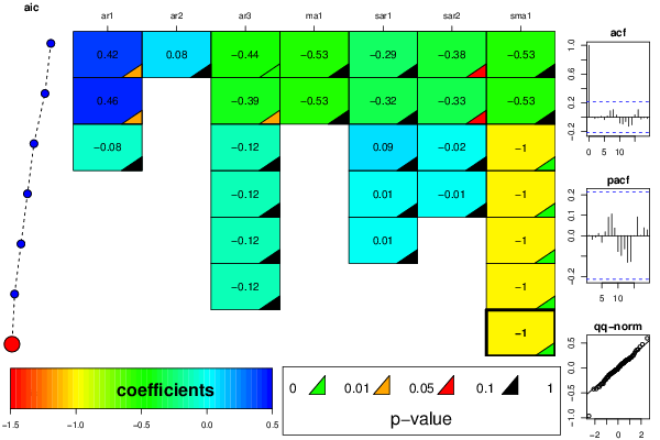
arimaSelectplot <- function(arimaSelect.out,noms,choix){
noms <- names(arimaSelect.out[[3]][[1]]$coef)
coeff <- arimaSelect.out[[1]]
k <- min(which(is.na(coeff[,1])))-1
coeff <- coeff[1:k,]
pval <- arimaSelect.out[[2]][1:k,]
aic <- arimaSelect.out$aic[1:k]
coeff[coeff==0] <- NA
n <- ncol(coeff)
if(missing(choix)) choix <- k
layout(matrix(c(1,1,1,2,
3,3,3,2,
3,3,3,4,
5,6,7,7),nr=4),
widths=c(10,35,45,15),
heights=c(30,30,15,15))
couleurs <- rainbow(75)[1:50]#(50)
ticks <- pretty(coeff)
par(mar=c(1,1,3,1))
plot(aic,k:1-.5,type='o',pch=21,bg='blue',cex=2,axes=F,lty=2,xpd=NA)
points(aic[choix],k-choix+.5,pch=21,cex=4,bg=2,xpd=NA)
title('aic',line=2)
par(mar=c(3,0,0,0))
plot(0,axes=F,xlab='',ylab='',xlim=range(ticks),ylim=c(.1,1))
rect(xleft = min(ticks) + (0:49)/50*(max(ticks)-min(ticks)),
xright = min(ticks) + (1:50)/50*(max(ticks)-min(ticks)),
ytop = rep(1,50),
ybottom= rep(0,50),col=couleurs,border=NA)
axis(1,ticks)
rect(xleft=min(ticks),xright=max(ticks),ytop=1,ybottom=0)
text(mean(coeff,na.rm=T),.5,'coefficients',cex=2,font=2)
par(mar=c(1,1,3,1))
image(1:n,1:k,t(coeff[k:1,]),axes=F,col=couleurs,zlim=range(ticks))
for(i in 1:n) for(j in 1:k) if(!is.na(coeff[j,i])) {
if(pval[j,i]<.01) symb = 'green'
else if( (pval[j,i]<.05) & (pval[j,i]>=.01)) symb = 'orange'
else if( (pval[j,i]<.1) & (pval[j,i]>=.05)) symb = 'red'
else symb = 'black'
polygon(c(i+.5 ,i+.2 ,i+.5 ,i+.5),
c(k-j+0.5,k-j+0.5,k-j+0.8,k-j+0.5),
col=symb)
if(j==choix) {
rect(xleft=i-.5,
xright=i+.5,
ybottom=k-j+1.5,
ytop=k-j+.5,
lwd=4)
text(i,
k-j+1,
round(coeff[j,i],2),
cex=1.2,
font=2)
}
else{
rect(xleft=i-.5,xright=i+.5,ybottom=k-j+1.5,ytop=k-j+.5)
text(i,k-j+1,round(coeff[j,i],2),cex=1.2,font=1)
}
}
axis(3,1:n,noms)
par(mar=c(0.5,0,0,0.5))
plot(0,axes=F,xlab='',ylab='',type='n',xlim=c(0,8),ylim=c(-.2,.8))
cols <- c('green','orange','red','black')
niv <- c('0','0.01','0.05','0.1')
for(i in 0:3){
polygon(c(1+2*i ,1+2*i ,1+2*i-.5 ,1+2*i),
c(.4 ,.7 , .4 , .4),
col=cols[i+1])
text(2*i,0.5,niv[i+1],cex=1.5)
}
text(8,.5,1,cex=1.5)
text(4,0,'p-value',cex=2)
box()
residus <- arimaSelect.out[[3]][[choix]]$res
par(mar=c(1,2,4,1))
acf(residus,main='')
title('acf',line=.5)
par(mar=c(1,2,4,1))
pacf(residus,main='')
title('pacf',line=.5)
par(mar=c(2,2,4,1))
qqnorm(residus,main='')
title('qq-norm',line=.5)
qqline(residus)
residus
}
if (par2 == 0) x <- log(x)
if (par2 != 0) x <- x^par2
(selection <- arimaSelect(x, order=c(par6,par3,par7), seasonal=list(order=c(par8,par4,par9), period=par5)))
bitmap(file='test1.png')
resid <- arimaSelectplot(selection)
dev.off()
resid
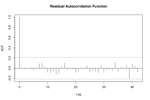
bitmap(file='test2.png')
acf(resid,length(resid)/2, main='Residual Autocorrelation Function')
dev.off()
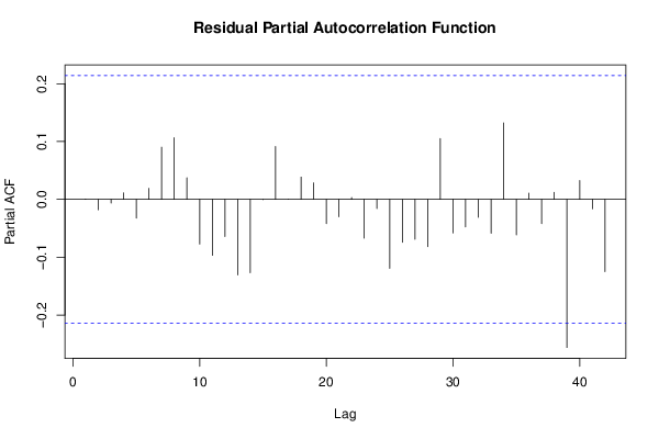
bitmap(file='test3.png')
pacf(resid,length(resid)/2, main='Residual Partial Autocorrelation Function')
dev.off()
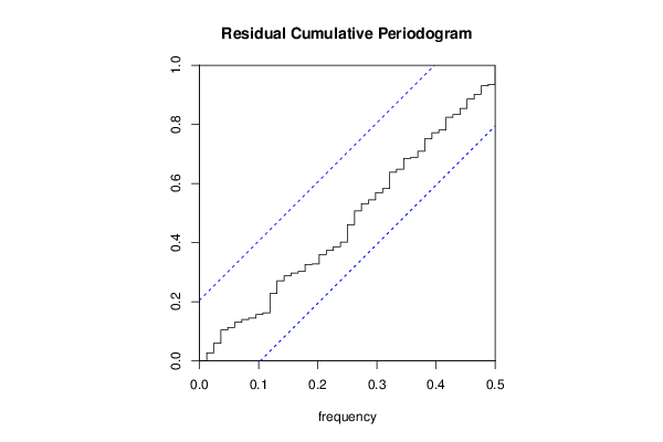
bitmap(file='test4.png')
cpgram(resid, main='Residual Cumulative Periodogram')
dev.off()
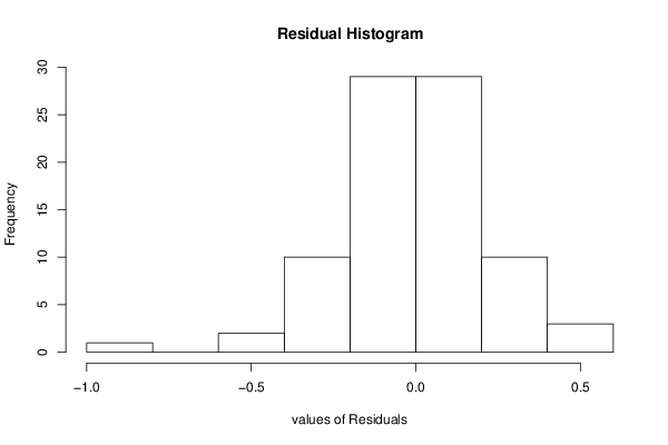
bitmap(file='test5.png')
hist(resid, main='Residual Histogram', xlab='values of Residuals')
dev.off()
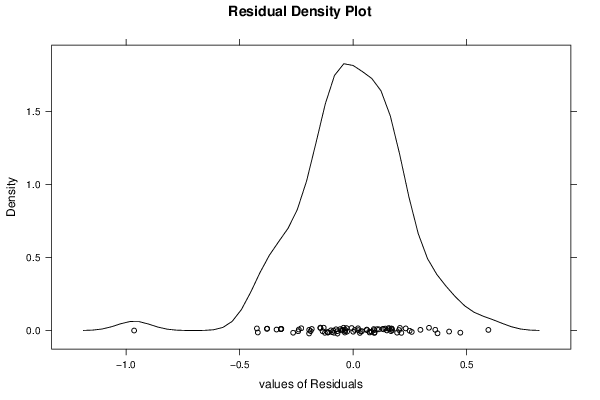
bitmap(file='test6.png')
densityplot(~resid,col='black',main='Residual Density Plot', xlab='values of Residuals')
dev.off()
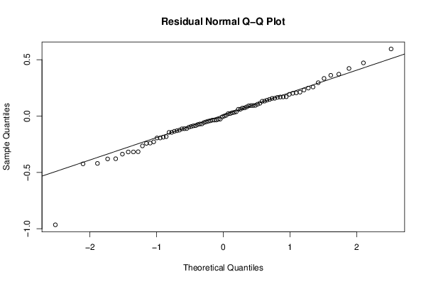
bitmap(file='test7.png')
qqnorm(resid, main='Residual Normal Q-Q Plot')
qqline(resid)
dev.off()
ncols <- length(selection[[1]][1,])
nrows <- length(selection[[2]][,1])-1
load(file='createtable')
a<-table.start()
a<-table.row.start(a)
a<-table.element(a,'ARIMA Parameter Estimation and Backward Selection', ncols+1,TRUE)
a<-table.row.end(a)
a<-table.row.start(a)
a<-table.element(a,'Iteration', header=TRUE)
for (i in 1:ncols) {
a<-table.element(a,names(selection[[3]][[1]]$coef)[i],header=TRUE)
}
a<-table.row.end(a)
for (j in 1:nrows) {
a<-table.row.start(a)
mydum <- 'Estimates ('
mydum <- paste(mydum,j)
mydum <- paste(mydum,')')
a<-table.element(a,mydum, header=TRUE)
for (i in 1:ncols) {
a<-table.element(a,round(selection[[1]][j,i],4))
}
a<-table.row.end(a)
a<-table.row.start(a)
a<-table.element(a,'(p-val)', header=TRUE)
for (i in 1:ncols) {
mydum <- '('
mydum <- paste(mydum,round(selection[[2]][j,i],4),sep='')
mydum <- paste(mydum,')')
a<-table.element(a,mydum)
}
a<-table.row.end(a)
}
a<-table.end(a)
table.save(a,file='mytable.tab')
a<-table.start()
a<-table.row.start(a)
a<-table.element(a,'Estimated ARIMA Residuals', 1,TRUE)
a<-table.row.end(a)
a<-table.row.start(a)
a<-table.element(a,'Value', 1,TRUE)
a<-table.row.end(a)
for (i in (par4*par5+par3):length(resid)) {
a<-table.row.start(a)
a<-table.element(a,resid[i])
a<-table.row.end(a)
}
a<-table.end(a)
table.save(a,file='mytable1.tab')