Repository of Reproducible Computations

Free Statistics

of Irreproducible Research!

Author's title

Author

*Unverified author*

R Software Module

rwasp_sdplot.wasp

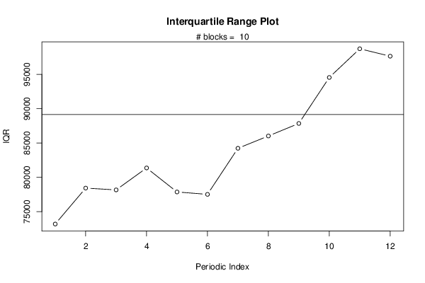
Title produced by software

Standard Deviation Plot

Date of computation

Sat, 23 Jul 2016 09:03:51 +0100

Cite this page as follows

Statistical Computations at FreeStatistics.org, Office for Research Development and Education, URL https://freestatistics.org/blog/index.php?v=date/2016/Jul/23/t1469261044b5gb1a7d2kxltdd.htm/, Retrieved Wed, 08 May 2024 02:31:39 +0000

Statistical Computations at FreeStatistics.org, Office for Research Development and Education, URL https://freestatistics.org/blog/index.php?pk=295933, Retrieved Wed, 08 May 2024 02:31:39 +0000

QR Codes:

Paste this QR Code to cite your computation.

Original text written by user:

IsPrivate?

No (this computation is public)

User-defined keywords

Estimated Impact

142

Family? (F = Feedback message, R = changed R code, M = changed R Module, P = changed Parameters, D = changed Data)

-       [Standard Deviation Plot] [] [2016-07-23 08:03:51] [d41d8cd98f00b204e9800998ecf8427e] [Current]

Feedback Forum

Post a new message

Dataseries X:

Download CSV

Histogram

Boxplots

Summary of computational transaction
Raw Input	view raw input (R code)
Raw Output	view raw output of R engine
Computing time	3 seconds
R Server	'Gwilym Jenkins' @ jenkins.wessa.net

\begin{tabular}{lllllllll}
\hline
Summary of computational transaction \tabularnewline
Raw Input & view raw input (R code)  \tabularnewline
Raw Output & view raw output of R engine  \tabularnewline
Computing time & 3 seconds \tabularnewline
R Server & 'Gwilym Jenkins' @ jenkins.wessa.net \tabularnewline
\hline
\end{tabular}
%Source: https://freestatistics.org/blog/index.php?pk=295933&T=0

[TABLE]
[ROW][C]Summary of computational transaction[/C][/ROW]
[ROW][C]Raw Input[/C][C]view raw input (R code) [/C][/ROW]
[ROW][C]Raw Output[/C][C]view raw output of R engine [/C][/ROW]
[ROW][C]Computing time[/C][C]3 seconds[/C][/ROW]
[ROW][C]R Server[/C][C]'Gwilym Jenkins' @ jenkins.wessa.net[/C][/ROW]
[/TABLE]
Source: https://freestatistics.org/blog/index.php?pk=295933&T=0

Globally Unique Identifier (entire table): ba.freestatistics.org/blog/index.php?pk=295933&T=0

As an alternative you can also use a QR Code:

The GUIDs for individual cells are displayed in the table below:

Summary of computational transaction
Raw Input	view raw input (R code)
Raw Output	view raw output of R engine
Computing time	3 seconds
R Server	'Gwilym Jenkins' @ jenkins.wessa.net

Figure 1

PNG link

Postscript link

PDF link

Figure 2

PNG link

Postscript link

PDF link

Figure 3

PNG link

Postscript link

PDF link

Figure 4

PNG link

Postscript link

PDF link

Figure 5

PNG link

Postscript link

PDF link

Figure 6

PNG link

Postscript link

PDF link

Parameters (Session):

par1 = 12 ;

Parameters (R input):

par1 = 12 ;

R code (references can be found in the software module):

par1 <- as.numeric(par1)
(n <- length(x))
(np <- floor(n / par1))
arr <- array(NA,dim=c(par1,np+1))
ari <- array(0,dim=par1)
j <- 0
for (i in 1:n)
{
j = j + 1
ari[j] = ari[j] + 1
arr[j,ari[j]] <- x[i]
if (j == par1) j = 0
}
ari
arr
arr.sd <- array(NA,dim=par1)
arr.range <- array(NA,dim=par1)
arr.iqr <- array(NA,dim=par1)
for (j in 1:par1)
{
arr.sd[j] <- sqrt(var(arr[j,],na.rm=TRUE))
arr.range[j] <- max(arr[j,],na.rm=TRUE) - min(arr[j,],na.rm=TRUE)
arr.iqr[j] <- quantile(arr[j,],0.75,na.rm=TRUE) - quantile(arr[j,],0.25,na.rm=TRUE)
}
overall.sd <- sqrt(var(x))
overall.range <- max(x) - min(x)
overall.iqr <- quantile(x,0.75) - quantile(x,0.25)
bitmap(file='plot1.png')
plot(arr.sd,type='b',ylab='S.D.',main='Standard Deviation Plot',xlab='Periodic Index')
mtext(paste('# blocks = ',np))
abline(overall.sd,0)
dev.off()
bitmap(file='plot2.png')
plot(arr.range,type='b',ylab='range',main='Range Plot',xlab='Periodic Index')
mtext(paste('# blocks = ',np))
abline(overall.range,0)
dev.off()
bitmap(file='plot3.png')
plot(arr.iqr,type='b',ylab='IQR',main='Interquartile Range Plot',xlab='Periodic Index')
mtext(paste('# blocks = ',np))
abline(overall.iqr,0)
dev.off()
bitmap(file='plot4.png')
z <- data.frame(t(arr))
names(z) <- c(1:par1)
(boxplot(z,notch=TRUE,col='grey',xlab='Periodic Index',ylab='Value',main='Notched Box Plots - Periodic Subseries'))
dev.off()
bitmap(file='plot5.png')
z <- data.frame(arr)
names(z) <- c(1:np)
(boxplot(z,notch=TRUE,col='grey',xlab='Block Index',ylab='Value',main='Notched Box Plots - Sequential Blocks'))
dev.off()
bitmap(file='plot6.png')
z <- data.frame(cbind(arr.sd,arr.range,arr.iqr))
names(z) <- list('S.D.','Range','IQR')
(boxplot(z,notch=TRUE,col='grey',ylab='Overall Variability',main='Notched Box Plots'))
dev.off()

Free Statistics

Description of Statistical Computation

Tree of Dependent Computations

Dataset

Tables (Output of Computation)

Figures (Output of Computation)

Input Parameters & R Code