Free Statistics
of Irreproducible Research!
Description of Statistical Computation | |||||||||||||||||||||
|---|---|---|---|---|---|---|---|---|---|---|---|---|---|---|---|---|---|---|---|---|---|
| Author's title | |||||||||||||||||||||
| Author | *Unverified author* | ||||||||||||||||||||
| R Software Module | rwasp_meanplot.wasp | ||||||||||||||||||||
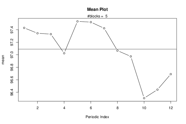
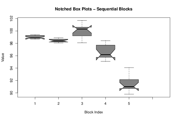
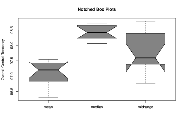
| Title produced by software | Mean Plot | ||||||||||||||||||||
| Date of computation | Sat, 05 Mar 2016 12:22:38 +0000 | ||||||||||||||||||||
| Cite this page as follows | Statistical Computations at FreeStatistics.org, Office for Research Development and Education, URL https://freestatistics.org/blog/index.php?v=date/2016/Mar/05/t1457180688544861d6xjg3q5i.htm/, Retrieved Sat, 27 Apr 2024 07:05:06 +0000 | ||||||||||||||||||||
| Statistical Computations at FreeStatistics.org, Office for Research Development and Education, URL https://freestatistics.org/blog/index.php?pk=293458, Retrieved Sat, 27 Apr 2024 07:05:06 +0000 | |||||||||||||||||||||
| QR Codes: | |||||||||||||||||||||
|
| |||||||||||||||||||||
| Original text written by user: | |||||||||||||||||||||
| IsPrivate? | No (this computation is public) | ||||||||||||||||||||
| User-defined keywords | |||||||||||||||||||||
| Estimated Impact | 99 | ||||||||||||||||||||
Tree of Dependent Computations | |||||||||||||||||||||
| Family? (F = Feedback message, R = changed R code, M = changed R Module, P = changed Parameters, D = changed Data) | |||||||||||||||||||||
| - [Central Tendency] [Studio 100 - Cent...] [2016-03-05 11:36:02] [e6773be784e85f51fb44487d8478f111] - RMPD [Mean Plot] [Mean plot Jaar G&...] [2016-03-05 12:12:35] [e6773be784e85f51fb44487d8478f111] - R PD [Mean Plot] [Mean plot Maand C...] [2016-03-05 12:22:38] [268d33ec1c95cc32f8abd6e0112b4a36] [Current] - R PD [Mean Plot] [Mean plot Jaar Co...] [2016-03-05 12:25:37] [e6773be784e85f51fb44487d8478f111] | |||||||||||||||||||||
| Feedback Forum | |||||||||||||||||||||
Post a new message | |||||||||||||||||||||
Dataset | |||||||||||||||||||||
| Dataseries X: | |||||||||||||||||||||
98,72 98,67 98,82 99,39 99,33 99,22 99,05 98,83 98,84 98,89 98,8 99,4 98,89 98,85 98,69 98,48 98,39 98,35 98,26 98,06 98,14 98,17 98,41 98,64 99,25 99,61 100,28 100,31 100,55 100,45 100,78 100,68 101,69 98,09 99,13 99,18 96,22 96,11 96 95,96 97,95 98,43 98,32 97,45 96,42 95,36 95,1 95,54 94,07 93,48 92,86 90,98 91,45 91,16 90,71 90,31 89,78 91,02 90,77 90,69 | |||||||||||||||||||||
Tables (Output of Computation) | |||||||||||||||||||||
| |||||||||||||||||||||
Figures (Output of Computation) | |||||||||||||||||||||
Input Parameters & R Code | |||||||||||||||||||||
| Parameters (Session): | |||||||||||||||||||||
| par1 = 12 ; | |||||||||||||||||||||
| Parameters (R input): | |||||||||||||||||||||
| par1 = 12 ; | |||||||||||||||||||||
| R code (references can be found in the software module): | |||||||||||||||||||||
par1 <- as.numeric(par1) | |||||||||||||||||||||