Free Statistics
of Irreproducible Research!
Description of Statistical Computation | |||||||||||||||||||||
|---|---|---|---|---|---|---|---|---|---|---|---|---|---|---|---|---|---|---|---|---|---|
| Author's title | |||||||||||||||||||||
| Author | *Unverified author* | ||||||||||||||||||||
| R Software Module | rwasp_meanplot.wasp | ||||||||||||||||||||
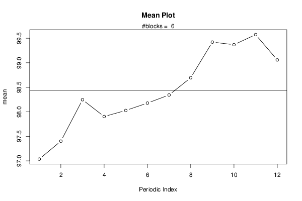
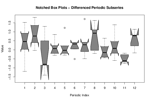
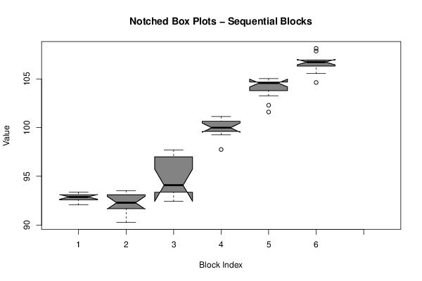
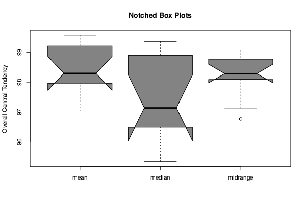
| Title produced by software | Mean Plot | ||||||||||||||||||||
| Date of computation | Sat, 05 Mar 2016 13:07:08 +0000 | ||||||||||||||||||||
| Cite this page as follows | Statistical Computations at FreeStatistics.org, Office for Research Development and Education, URL https://freestatistics.org/blog/index.php?v=date/2016/Mar/05/t1457183260eahimx4ysi4z7du.htm/, Retrieved Sat, 27 Apr 2024 07:24:27 +0000 | ||||||||||||||||||||
| Statistical Computations at FreeStatistics.org, Office for Research Development and Education, URL https://freestatistics.org/blog/index.php?pk=293467, Retrieved Sat, 27 Apr 2024 07:24:27 +0000 | |||||||||||||||||||||
| QR Codes: | |||||||||||||||||||||
|
| |||||||||||||||||||||
| Original text written by user: | |||||||||||||||||||||
| IsPrivate? | No (this computation is public) | ||||||||||||||||||||
| User-defined keywords | |||||||||||||||||||||
| Estimated Impact | 94 | ||||||||||||||||||||
Tree of Dependent Computations | |||||||||||||||||||||
| Family? (F = Feedback message, R = changed R code, M = changed R Module, P = changed Parameters, D = changed Data) | |||||||||||||||||||||
| - [Mean Plot] [Opdracht 6/oef2] [2016-03-05 13:07:08] [efea2b8bc7c91838390b884e612c3e3f] [Current] | |||||||||||||||||||||
| Feedback Forum | |||||||||||||||||||||
Post a new message | |||||||||||||||||||||
Dataset | |||||||||||||||||||||
| Dataseries X: | |||||||||||||||||||||
92,94 92,97 93,37 92,6 92,84 92,55 92,93 92,44 93,36 93,24 92,65 92,06 92,88 91,69 91,66 90,26 91,11 92,33 91,82 92,24 93,35 93,53 93,34 92,59 92,42 92,64 94,44 93,59 93,39 93,33 93,72 95,43 97,06 97,7 97,59 96,97 97,75 99,27 100,63 99,8 99,5 99,72 99,77 100,18 101,11 100,67 101,13 100,46 101,6 102,3 103,26 104,56 104,61 104,62 105,03 104,93 104,73 104,33 104,6 104,41 104,63 105,55 106,12 106,62 106,72 106,52 106,79 106,95 106,92 106,74 108,13 107,86 | |||||||||||||||||||||
Tables (Output of Computation) | |||||||||||||||||||||
| |||||||||||||||||||||
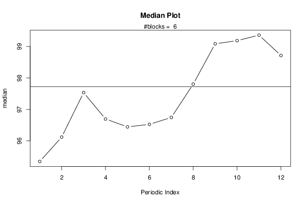
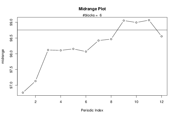
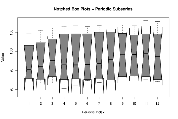
Figures (Output of Computation) | |||||||||||||||||||||
Input Parameters & R Code | |||||||||||||||||||||
| Parameters (Session): | |||||||||||||||||||||
| par1 = 12 ; | |||||||||||||||||||||
| Parameters (R input): | |||||||||||||||||||||
| par1 = 12 ; | |||||||||||||||||||||
| R code (references can be found in the software module): | |||||||||||||||||||||
par1 <- as.numeric(par1) | |||||||||||||||||||||