Free Statistics
of Irreproducible Research!
Description of Statistical Computation | |||||||||||||||||||||
|---|---|---|---|---|---|---|---|---|---|---|---|---|---|---|---|---|---|---|---|---|---|
| Author's title | |||||||||||||||||||||
| Author | *Unverified author* | ||||||||||||||||||||
| R Software Module | rwasp_meanplot.wasp | ||||||||||||||||||||
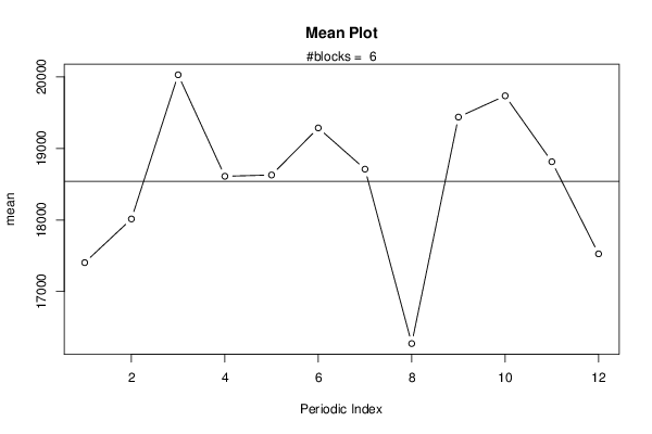
| Title produced by software | Mean Plot | ||||||||||||||||||||
| Date of computation | Mon, 07 Mar 2016 15:13:13 +0000 | ||||||||||||||||||||
| Cite this page as follows | Statistical Computations at FreeStatistics.org, Office for Research Development and Education, URL https://freestatistics.org/blog/index.php?v=date/2016/Mar/07/t1457363754ds3u2db2xc9u8lg.htm/, Retrieved Wed, 01 May 2024 08:54:00 +0000 | ||||||||||||||||||||
| Statistical Computations at FreeStatistics.org, Office for Research Development and Education, URL https://freestatistics.org/blog/index.php?pk=293580, Retrieved Wed, 01 May 2024 08:54:00 +0000 | |||||||||||||||||||||
| QR Codes: | |||||||||||||||||||||
|
| |||||||||||||||||||||
| Original text written by user: | |||||||||||||||||||||
| IsPrivate? | No (this computation is public) | ||||||||||||||||||||
| User-defined keywords | |||||||||||||||||||||
| Estimated Impact | 109 | ||||||||||||||||||||
Tree of Dependent Computations | |||||||||||||||||||||
| Family? (F = Feedback message, R = changed R code, M = changed R Module, P = changed Parameters, D = changed Data) | |||||||||||||||||||||
| - [Mean Plot] [Uitvoer Belgi�] [2016-03-07 15:13:13] [30ac29e28bcab64021946a7872e1db5d] [Current] | |||||||||||||||||||||
| Feedback Forum | |||||||||||||||||||||
Post a new message | |||||||||||||||||||||
Dataset | |||||||||||||||||||||
| Dataseries X: | |||||||||||||||||||||
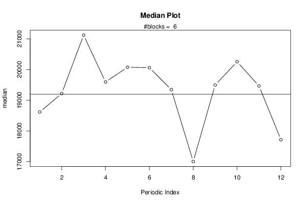
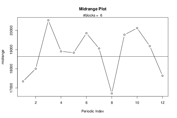
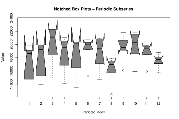
13566,7 13941,5 14964,1 14086 13505,1 15300,4 14725,2 12484,9 16082,6 15915,8 15916,1 15713 14746 15253,2 18384,3 16848,5 16485,5 19257,1 17093,4 15700,1 19124,3 18640,8 18439,2 17106,3 18347,7 19372,7 22263,8 19422,9 21268,6 20310 19256 17535,9 19857,4 19628,4 19727,5 18112,2 18889,3 20516,1 22317 19768,8 20015,8 20260,5 19434,3 17910 19134,4 20880,1 19680 17493,4 19087,8 19064,6 21191 20503,9 20364,1 19860,4 20924,1 17018,8 20607,4 21500,2 19868,3 18801,9 19787,5 19936,2 21047,6 21034,4 20132,8 20725,3 20827,8 16992,3 21818,2 21841,4 19252,2 17933,7 | |||||||||||||||||||||
Tables (Output of Computation) | |||||||||||||||||||||
| |||||||||||||||||||||
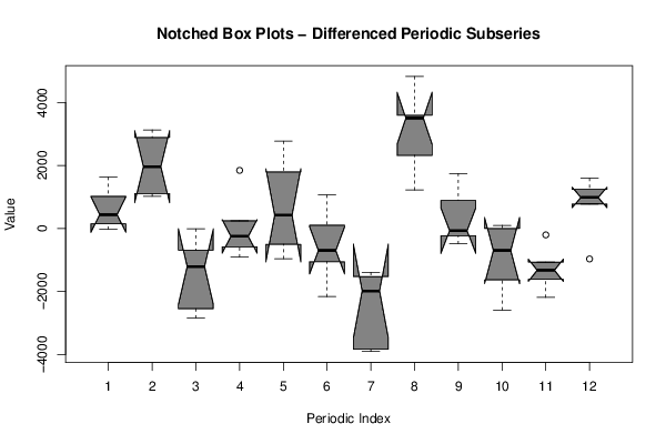
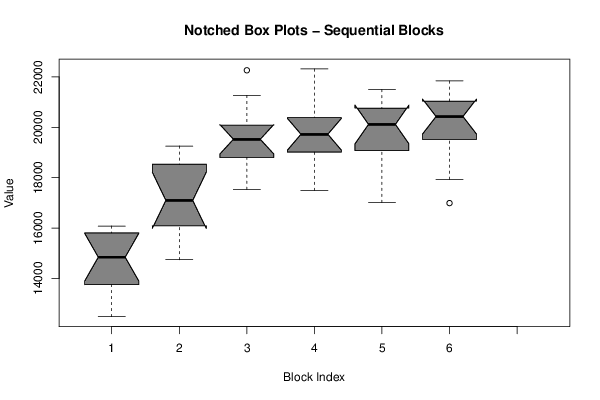
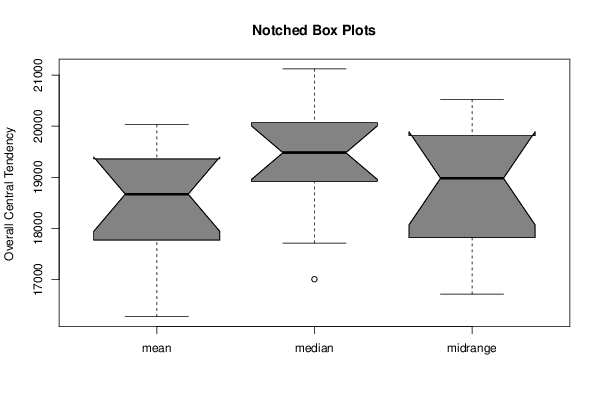
Figures (Output of Computation) | |||||||||||||||||||||
Input Parameters & R Code | |||||||||||||||||||||
| Parameters (Session): | |||||||||||||||||||||
| par1 = 12 ; | |||||||||||||||||||||
| Parameters (R input): | |||||||||||||||||||||
| par1 = 12 ; | |||||||||||||||||||||
| R code (references can be found in the software module): | |||||||||||||||||||||
par1 <- as.numeric(par1) | |||||||||||||||||||||