Repository of Reproducible Computations

Free Statistics

of Irreproducible Research!

Author's title

Author

*Unverified author*

R Software Module

rwasp_autocorrelation.wasp

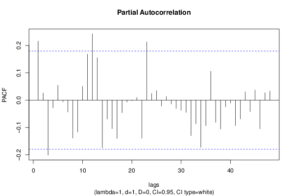
Title produced by software

(Partial) Autocorrelation Function

Date of computation

Thu, 10 Mar 2016 15:49:05 +0000

Cite this page as follows

Statistical Computations at FreeStatistics.org, Office for Research Development and Education, URL https://freestatistics.org/blog/index.php?v=date/2016/Mar/10/t1457625063exk7ef3npcd33q5.htm/, Retrieved Wed, 08 May 2024 03:43:13 +0000

Statistical Computations at FreeStatistics.org, Office for Research Development and Education, URL https://freestatistics.org/blog/index.php?pk=293845, Retrieved Wed, 08 May 2024 03:43:13 +0000

QR Codes:

Paste this QR Code to cite your computation.

Original text written by user:

IsPrivate?

No (this computation is public)

User-defined keywords

Estimated Impact

165

Family? (F = Feedback message, R = changed R code, M = changed R Module, P = changed Parameters, D = changed Data)

-       [(Partial) Autocorrelation Function] [consumptieprijsin...] [2016-03-10 15:49:05] [567a9be58124adae7ccc8a0c8709ba48] [Current]

Feedback Forum

Post a new message

Dataseries X:

Download CSV

Histogram

Boxplots

Summary of computational transaction
Raw Input	view raw input (R code)
Raw Output	view raw output of R engine
Computing time	2 seconds
R Server	'Gwilym Jenkins' @ jenkins.wessa.net

\begin{tabular}{lllllllll}
\hline
Summary of computational transaction \tabularnewline
Raw Input & view raw input (R code)  \tabularnewline
Raw Output & view raw output of R engine  \tabularnewline
Computing time & 2 seconds \tabularnewline
R Server & 'Gwilym Jenkins' @ jenkins.wessa.net \tabularnewline
\hline
\end{tabular}
%Source: https://freestatistics.org/blog/index.php?pk=293845&T=0

[TABLE]
[ROW][C]Summary of computational transaction[/C][/ROW]
[ROW][C]Raw Input[/C][C]view raw input (R code) [/C][/ROW]
[ROW][C]Raw Output[/C][C]view raw output of R engine [/C][/ROW]
[ROW][C]Computing time[/C][C]2 seconds[/C][/ROW]
[ROW][C]R Server[/C][C]'Gwilym Jenkins' @ jenkins.wessa.net[/C][/ROW]
[/TABLE]
Source: https://freestatistics.org/blog/index.php?pk=293845&T=0

Globally Unique Identifier (entire table): ba.freestatistics.org/blog/index.php?pk=293845&T=0

As an alternative you can also use a QR Code:

The GUIDs for individual cells are displayed in the table below:

Summary of computational transaction
Raw Input	view raw input (R code)
Raw Output	view raw output of R engine
Computing time	2 seconds
R Server	'Gwilym Jenkins' @ jenkins.wessa.net

Autocorrelation Function
Time lag k	ACF(k)	T-STAT	P-value
1	0.216148	2.3579	0.010005
2	0.071792	0.7832	0.217545
3	-0.170872	-1.864	0.032394
4	-0.101322	-1.1053	0.135631
5	-0.00388	-0.0423	0.483156
6	0.028083	0.3064	0.379935
7	-0.004599	-0.0502	0.480035
8	-0.138259	-1.5082	0.067074
9	-0.17469	-1.9056	0.029555
10	-0.032569	-0.3553	0.361503
11	0.174849	1.9074	0.029441
12	0.343116	3.743	0.000141
13	0.273176	2.98	0.001748
14	-0.077126	-0.8413	0.200922
15	-0.145584	-1.5881	0.057455
16	-0.20418	-2.2273	0.013903
17	-0.120085	-1.31	0.096365
18	-0.034696	-0.3785	0.352869
19	-0.032425	-0.3537	0.362088
20	-0.087098	-0.9501	0.171986
21	-0.127191	-1.3875	0.083943
22	-0.146648	-1.5997	0.056154
23	0.238501	2.6017	0.005226
24	0.229784	2.5066	0.006769
25	0.262883	2.8677	0.002446
26	-0.007673	-0.0837	0.466718
27	-0.107522	-1.1729	0.121583
28	-0.144129	-1.5723	0.059273
29	-0.113338	-1.2364	0.109379
30	-0.024017	-0.262	0.396887
31	-0.040047	-0.4369	0.331503
32	-0.142778	-1.5575	0.061001
33	-0.16755	-1.8278	0.035046
34	-0.196105	-2.1393	0.017229
35	0.01271	0.1386	0.444981
36	0.278607	3.0392	0.001458
37	0.108062	1.1788	0.120411
38	-0.00362	-0.0395	0.484282
39	-0.163096	-1.7792	0.038883
40	-0.134404	-1.4662	0.07262
41	-0.143879	-1.5695	0.05959
42	-0.061973	-0.676	0.250161
43	0.013852	0.1511	0.440074
44	-0.093714	-1.0223	0.154358
45	-0.1217	-1.3276	0.093427
46	-0.129928	-1.4173	0.079498
47	0.047965	0.5232	0.300891
48	0.257754	2.8118	0.002882

\begin{tabular}{lllllllll}
\hline
Autocorrelation Function \tabularnewline
Time lag k & ACF(k) & T-STAT & P-value \tabularnewline
1 & 0.216148 & 2.3579 & 0.010005 \tabularnewline
2 & 0.071792 & 0.7832 & 0.217545 \tabularnewline
3 & -0.170872 & -1.864 & 0.032394 \tabularnewline
4 & -0.101322 & -1.1053 & 0.135631 \tabularnewline
5 & -0.00388 & -0.0423 & 0.483156 \tabularnewline
6 & 0.028083 & 0.3064 & 0.379935 \tabularnewline
7 & -0.004599 & -0.0502 & 0.480035 \tabularnewline
8 & -0.138259 & -1.5082 & 0.067074 \tabularnewline
9 & -0.17469 & -1.9056 & 0.029555 \tabularnewline
10 & -0.032569 & -0.3553 & 0.361503 \tabularnewline
11 & 0.174849 & 1.9074 & 0.029441 \tabularnewline
12 & 0.343116 & 3.743 & 0.000141 \tabularnewline
13 & 0.273176 & 2.98 & 0.001748 \tabularnewline
14 & -0.077126 & -0.8413 & 0.200922 \tabularnewline
15 & -0.145584 & -1.5881 & 0.057455 \tabularnewline
16 & -0.20418 & -2.2273 & 0.013903 \tabularnewline
17 & -0.120085 & -1.31 & 0.096365 \tabularnewline
18 & -0.034696 & -0.3785 & 0.352869 \tabularnewline
19 & -0.032425 & -0.3537 & 0.362088 \tabularnewline
20 & -0.087098 & -0.9501 & 0.171986 \tabularnewline
21 & -0.127191 & -1.3875 & 0.083943 \tabularnewline
22 & -0.146648 & -1.5997 & 0.056154 \tabularnewline
23 & 0.238501 & 2.6017 & 0.005226 \tabularnewline
24 & 0.229784 & 2.5066 & 0.006769 \tabularnewline
25 & 0.262883 & 2.8677 & 0.002446 \tabularnewline
26 & -0.007673 & -0.0837 & 0.466718 \tabularnewline
27 & -0.107522 & -1.1729 & 0.121583 \tabularnewline
28 & -0.144129 & -1.5723 & 0.059273 \tabularnewline
29 & -0.113338 & -1.2364 & 0.109379 \tabularnewline
30 & -0.024017 & -0.262 & 0.396887 \tabularnewline
31 & -0.040047 & -0.4369 & 0.331503 \tabularnewline
32 & -0.142778 & -1.5575 & 0.061001 \tabularnewline
33 & -0.16755 & -1.8278 & 0.035046 \tabularnewline
34 & -0.196105 & -2.1393 & 0.017229 \tabularnewline
35 & 0.01271 & 0.1386 & 0.444981 \tabularnewline
36 & 0.278607 & 3.0392 & 0.001458 \tabularnewline
37 & 0.108062 & 1.1788 & 0.120411 \tabularnewline
38 & -0.00362 & -0.0395 & 0.484282 \tabularnewline
39 & -0.163096 & -1.7792 & 0.038883 \tabularnewline
40 & -0.134404 & -1.4662 & 0.07262 \tabularnewline
41 & -0.143879 & -1.5695 & 0.05959 \tabularnewline
42 & -0.061973 & -0.676 & 0.250161 \tabularnewline
43 & 0.013852 & 0.1511 & 0.440074 \tabularnewline
44 & -0.093714 & -1.0223 & 0.154358 \tabularnewline
45 & -0.1217 & -1.3276 & 0.093427 \tabularnewline
46 & -0.129928 & -1.4173 & 0.079498 \tabularnewline
47 & 0.047965 & 0.5232 & 0.300891 \tabularnewline
48 & 0.257754 & 2.8118 & 0.002882 \tabularnewline
\hline
\end{tabular}
%Source: https://freestatistics.org/blog/index.php?pk=293845&T=1

[TABLE]
[ROW][C]Autocorrelation Function[/C][/ROW]
[ROW][C]Time lag k[/C][C]ACF(k)[/C][C]T-STAT[/C][C]P-value[/C][/ROW]
[ROW][C]1[/C][C]0.216148[/C][C]2.3579[/C][C]0.010005[/C][/ROW]
[ROW][C]2[/C][C]0.071792[/C][C]0.7832[/C][C]0.217545[/C][/ROW]
[ROW][C]3[/C][C]-0.170872[/C][C]-1.864[/C][C]0.032394[/C][/ROW]
[ROW][C]4[/C][C]-0.101322[/C][C]-1.1053[/C][C]0.135631[/C][/ROW]
[ROW][C]5[/C][C]-0.00388[/C][C]-0.0423[/C][C]0.483156[/C][/ROW]
[ROW][C]6[/C][C]0.028083[/C][C]0.3064[/C][C]0.379935[/C][/ROW]
[ROW][C]7[/C][C]-0.004599[/C][C]-0.0502[/C][C]0.480035[/C][/ROW]
[ROW][C]8[/C][C]-0.138259[/C][C]-1.5082[/C][C]0.067074[/C][/ROW]
[ROW][C]9[/C][C]-0.17469[/C][C]-1.9056[/C][C]0.029555[/C][/ROW]
[ROW][C]10[/C][C]-0.032569[/C][C]-0.3553[/C][C]0.361503[/C][/ROW]
[ROW][C]11[/C][C]0.174849[/C][C]1.9074[/C][C]0.029441[/C][/ROW]
[ROW][C]12[/C][C]0.343116[/C][C]3.743[/C][C]0.000141[/C][/ROW]
[ROW][C]13[/C][C]0.273176[/C][C]2.98[/C][C]0.001748[/C][/ROW]
[ROW][C]14[/C][C]-0.077126[/C][C]-0.8413[/C][C]0.200922[/C][/ROW]
[ROW][C]15[/C][C]-0.145584[/C][C]-1.5881[/C][C]0.057455[/C][/ROW]
[ROW][C]16[/C][C]-0.20418[/C][C]-2.2273[/C][C]0.013903[/C][/ROW]
[ROW][C]17[/C][C]-0.120085[/C][C]-1.31[/C][C]0.096365[/C][/ROW]
[ROW][C]18[/C][C]-0.034696[/C][C]-0.3785[/C][C]0.352869[/C][/ROW]
[ROW][C]19[/C][C]-0.032425[/C][C]-0.3537[/C][C]0.362088[/C][/ROW]
[ROW][C]20[/C][C]-0.087098[/C][C]-0.9501[/C][C]0.171986[/C][/ROW]
[ROW][C]21[/C][C]-0.127191[/C][C]-1.3875[/C][C]0.083943[/C][/ROW]
[ROW][C]22[/C][C]-0.146648[/C][C]-1.5997[/C][C]0.056154[/C][/ROW]
[ROW][C]23[/C][C]0.238501[/C][C]2.6017[/C][C]0.005226[/C][/ROW]
[ROW][C]24[/C][C]0.229784[/C][C]2.5066[/C][C]0.006769[/C][/ROW]
[ROW][C]25[/C][C]0.262883[/C][C]2.8677[/C][C]0.002446[/C][/ROW]
[ROW][C]26[/C][C]-0.007673[/C][C]-0.0837[/C][C]0.466718[/C][/ROW]
[ROW][C]27[/C][C]-0.107522[/C][C]-1.1729[/C][C]0.121583[/C][/ROW]
[ROW][C]28[/C][C]-0.144129[/C][C]-1.5723[/C][C]0.059273[/C][/ROW]
[ROW][C]29[/C][C]-0.113338[/C][C]-1.2364[/C][C]0.109379[/C][/ROW]
[ROW][C]30[/C][C]-0.024017[/C][C]-0.262[/C][C]0.396887[/C][/ROW]
[ROW][C]31[/C][C]-0.040047[/C][C]-0.4369[/C][C]0.331503[/C][/ROW]
[ROW][C]32[/C][C]-0.142778[/C][C]-1.5575[/C][C]0.061001[/C][/ROW]
[ROW][C]33[/C][C]-0.16755[/C][C]-1.8278[/C][C]0.035046[/C][/ROW]
[ROW][C]34[/C][C]-0.196105[/C][C]-2.1393[/C][C]0.017229[/C][/ROW]
[ROW][C]35[/C][C]0.01271[/C][C]0.1386[/C][C]0.444981[/C][/ROW]
[ROW][C]36[/C][C]0.278607[/C][C]3.0392[/C][C]0.001458[/C][/ROW]
[ROW][C]37[/C][C]0.108062[/C][C]1.1788[/C][C]0.120411[/C][/ROW]
[ROW][C]38[/C][C]-0.00362[/C][C]-0.0395[/C][C]0.484282[/C][/ROW]
[ROW][C]39[/C][C]-0.163096[/C][C]-1.7792[/C][C]0.038883[/C][/ROW]
[ROW][C]40[/C][C]-0.134404[/C][C]-1.4662[/C][C]0.07262[/C][/ROW]
[ROW][C]41[/C][C]-0.143879[/C][C]-1.5695[/C][C]0.05959[/C][/ROW]
[ROW][C]42[/C][C]-0.061973[/C][C]-0.676[/C][C]0.250161[/C][/ROW]
[ROW][C]43[/C][C]0.013852[/C][C]0.1511[/C][C]0.440074[/C][/ROW]
[ROW][C]44[/C][C]-0.093714[/C][C]-1.0223[/C][C]0.154358[/C][/ROW]
[ROW][C]45[/C][C]-0.1217[/C][C]-1.3276[/C][C]0.093427[/C][/ROW]
[ROW][C]46[/C][C]-0.129928[/C][C]-1.4173[/C][C]0.079498[/C][/ROW]
[ROW][C]47[/C][C]0.047965[/C][C]0.5232[/C][C]0.300891[/C][/ROW]
[ROW][C]48[/C][C]0.257754[/C][C]2.8118[/C][C]0.002882[/C][/ROW]
[/TABLE]
Source: https://freestatistics.org/blog/index.php?pk=293845&T=1

Globally Unique Identifier (entire table): ba.freestatistics.org/blog/index.php?pk=293845&T=1

As an alternative you can also use a QR Code:

The GUIDs for individual cells are displayed in the table below:

Autocorrelation Function
Time lag k	ACF(k)	T-STAT	P-value
1	0.216148	2.3579	0.010005
2	0.071792	0.7832	0.217545
3	-0.170872	-1.864	0.032394
4	-0.101322	-1.1053	0.135631
5	-0.00388	-0.0423	0.483156
6	0.028083	0.3064	0.379935
7	-0.004599	-0.0502	0.480035
8	-0.138259	-1.5082	0.067074
9	-0.17469	-1.9056	0.029555
10	-0.032569	-0.3553	0.361503
11	0.174849	1.9074	0.029441
12	0.343116	3.743	0.000141
13	0.273176	2.98	0.001748
14	-0.077126	-0.8413	0.200922
15	-0.145584	-1.5881	0.057455
16	-0.20418	-2.2273	0.013903
17	-0.120085	-1.31	0.096365
18	-0.034696	-0.3785	0.352869
19	-0.032425	-0.3537	0.362088
20	-0.087098	-0.9501	0.171986
21	-0.127191	-1.3875	0.083943
22	-0.146648	-1.5997	0.056154
23	0.238501	2.6017	0.005226
24	0.229784	2.5066	0.006769
25	0.262883	2.8677	0.002446
26	-0.007673	-0.0837	0.466718
27	-0.107522	-1.1729	0.121583
28	-0.144129	-1.5723	0.059273
29	-0.113338	-1.2364	0.109379
30	-0.024017	-0.262	0.396887
31	-0.040047	-0.4369	0.331503
32	-0.142778	-1.5575	0.061001
33	-0.16755	-1.8278	0.035046
34	-0.196105	-2.1393	0.017229
35	0.01271	0.1386	0.444981
36	0.278607	3.0392	0.001458
37	0.108062	1.1788	0.120411
38	-0.00362	-0.0395	0.484282
39	-0.163096	-1.7792	0.038883
40	-0.134404	-1.4662	0.07262
41	-0.143879	-1.5695	0.05959
42	-0.061973	-0.676	0.250161
43	0.013852	0.1511	0.440074
44	-0.093714	-1.0223	0.154358
45	-0.1217	-1.3276	0.093427
46	-0.129928	-1.4173	0.079498
47	0.047965	0.5232	0.300891
48	0.257754	2.8118	0.002882

Partial Autocorrelation Function
Time lag k	PACF(k)	T-STAT	P-value
1	0.216148	2.3579	0.010005
2	0.026301	0.2869	0.387342
3	-0.201199	-2.1948	0.015059
4	-0.02833	-0.309	0.378915
5	0.054301	0.5924	0.277369
6	-0.006308	-0.0688	0.472628
7	-0.043765	-0.4774	0.316969
8	-0.138541	-1.5113	0.066681
9	-0.116699	-1.273	0.102743
10	0.050439	0.5502	0.291597
11	0.168205	1.8349	0.034509
12	0.242704	2.6476	0.004603
13	0.155214	1.6932	0.046518
14	-0.17414	-1.8996	0.02995
15	-0.069093	-0.7537	0.226254
16	-0.10438	-1.1387	0.128567
17	-0.140207	-1.5295	0.064401
18	-0.045823	-0.4999	0.309044
19	-0.006858	-0.0748	0.470246
20	-0.002197	-0.024	0.490459
21	0.009519	0.1038	0.458737
22	-0.139151	-1.518	0.065838
23	0.213186	2.3256	0.010867
24	0.024668	0.2691	0.394162
25	0.034674	0.3782	0.35296
26	-0.021664	-0.2363	0.406791
27	0.013195	0.1439	0.442895
28	-0.014309	-0.1561	0.438112
29	-0.030172	-0.3291	0.371313
30	-0.037193	-0.4057	0.342835
31	-0.044885	-0.4896	0.312644
32	-0.129974	-1.4178	0.079424
33	-0.086951	-0.9485	0.172392
34	-0.172131	-1.8777	0.031433
35	-0.093559	-1.0206	0.154754
36	0.106034	1.1567	0.124858
37	-0.081284	-0.8867	0.188513
38	-0.105606	-1.152	0.125809
39	-0.024711	-0.2696	0.393982
40	-0.010481	-0.1143	0.454581
41	-0.09354	-1.0204	0.154805
42	-0.068612	-0.7485	0.227826
43	0.03026	0.3301	0.370952
44	-0.041959	-0.4577	0.323996
45	0.037077	0.4045	0.3433
46	-0.104912	-1.1445	0.127366
47	0.027243	0.2972	0.383423
48	0.033212	0.3623	0.358885

\begin{tabular}{lllllllll}
\hline
Partial Autocorrelation Function \tabularnewline
Time lag k & PACF(k) & T-STAT & P-value \tabularnewline
1 & 0.216148 & 2.3579 & 0.010005 \tabularnewline
2 & 0.026301 & 0.2869 & 0.387342 \tabularnewline
3 & -0.201199 & -2.1948 & 0.015059 \tabularnewline
4 & -0.02833 & -0.309 & 0.378915 \tabularnewline
5 & 0.054301 & 0.5924 & 0.277369 \tabularnewline
6 & -0.006308 & -0.0688 & 0.472628 \tabularnewline
7 & -0.043765 & -0.4774 & 0.316969 \tabularnewline
8 & -0.138541 & -1.5113 & 0.066681 \tabularnewline
9 & -0.116699 & -1.273 & 0.102743 \tabularnewline
10 & 0.050439 & 0.5502 & 0.291597 \tabularnewline
11 & 0.168205 & 1.8349 & 0.034509 \tabularnewline
12 & 0.242704 & 2.6476 & 0.004603 \tabularnewline
13 & 0.155214 & 1.6932 & 0.046518 \tabularnewline
14 & -0.17414 & -1.8996 & 0.02995 \tabularnewline
15 & -0.069093 & -0.7537 & 0.226254 \tabularnewline
16 & -0.10438 & -1.1387 & 0.128567 \tabularnewline
17 & -0.140207 & -1.5295 & 0.064401 \tabularnewline
18 & -0.045823 & -0.4999 & 0.309044 \tabularnewline
19 & -0.006858 & -0.0748 & 0.470246 \tabularnewline
20 & -0.002197 & -0.024 & 0.490459 \tabularnewline
21 & 0.009519 & 0.1038 & 0.458737 \tabularnewline
22 & -0.139151 & -1.518 & 0.065838 \tabularnewline
23 & 0.213186 & 2.3256 & 0.010867 \tabularnewline
24 & 0.024668 & 0.2691 & 0.394162 \tabularnewline
25 & 0.034674 & 0.3782 & 0.35296 \tabularnewline
26 & -0.021664 & -0.2363 & 0.406791 \tabularnewline
27 & 0.013195 & 0.1439 & 0.442895 \tabularnewline
28 & -0.014309 & -0.1561 & 0.438112 \tabularnewline
29 & -0.030172 & -0.3291 & 0.371313 \tabularnewline
30 & -0.037193 & -0.4057 & 0.342835 \tabularnewline
31 & -0.044885 & -0.4896 & 0.312644 \tabularnewline
32 & -0.129974 & -1.4178 & 0.079424 \tabularnewline
33 & -0.086951 & -0.9485 & 0.172392 \tabularnewline
34 & -0.172131 & -1.8777 & 0.031433 \tabularnewline
35 & -0.093559 & -1.0206 & 0.154754 \tabularnewline
36 & 0.106034 & 1.1567 & 0.124858 \tabularnewline
37 & -0.081284 & -0.8867 & 0.188513 \tabularnewline
38 & -0.105606 & -1.152 & 0.125809 \tabularnewline
39 & -0.024711 & -0.2696 & 0.393982 \tabularnewline
40 & -0.010481 & -0.1143 & 0.454581 \tabularnewline
41 & -0.09354 & -1.0204 & 0.154805 \tabularnewline
42 & -0.068612 & -0.7485 & 0.227826 \tabularnewline
43 & 0.03026 & 0.3301 & 0.370952 \tabularnewline
44 & -0.041959 & -0.4577 & 0.323996 \tabularnewline
45 & 0.037077 & 0.4045 & 0.3433 \tabularnewline
46 & -0.104912 & -1.1445 & 0.127366 \tabularnewline
47 & 0.027243 & 0.2972 & 0.383423 \tabularnewline
48 & 0.033212 & 0.3623 & 0.358885 \tabularnewline
\hline
\end{tabular}
%Source: https://freestatistics.org/blog/index.php?pk=293845&T=2

[TABLE]
[ROW][C]Partial Autocorrelation Function[/C][/ROW]
[ROW][C]Time lag k[/C][C]PACF(k)[/C][C]T-STAT[/C][C]P-value[/C][/ROW]
[ROW][C]1[/C][C]0.216148[/C][C]2.3579[/C][C]0.010005[/C][/ROW]
[ROW][C]2[/C][C]0.026301[/C][C]0.2869[/C][C]0.387342[/C][/ROW]
[ROW][C]3[/C][C]-0.201199[/C][C]-2.1948[/C][C]0.015059[/C][/ROW]
[ROW][C]4[/C][C]-0.02833[/C][C]-0.309[/C][C]0.378915[/C][/ROW]
[ROW][C]5[/C][C]0.054301[/C][C]0.5924[/C][C]0.277369[/C][/ROW]
[ROW][C]6[/C][C]-0.006308[/C][C]-0.0688[/C][C]0.472628[/C][/ROW]
[ROW][C]7[/C][C]-0.043765[/C][C]-0.4774[/C][C]0.316969[/C][/ROW]
[ROW][C]8[/C][C]-0.138541[/C][C]-1.5113[/C][C]0.066681[/C][/ROW]
[ROW][C]9[/C][C]-0.116699[/C][C]-1.273[/C][C]0.102743[/C][/ROW]
[ROW][C]10[/C][C]0.050439[/C][C]0.5502[/C][C]0.291597[/C][/ROW]
[ROW][C]11[/C][C]0.168205[/C][C]1.8349[/C][C]0.034509[/C][/ROW]
[ROW][C]12[/C][C]0.242704[/C][C]2.6476[/C][C]0.004603[/C][/ROW]
[ROW][C]13[/C][C]0.155214[/C][C]1.6932[/C][C]0.046518[/C][/ROW]
[ROW][C]14[/C][C]-0.17414[/C][C]-1.8996[/C][C]0.02995[/C][/ROW]
[ROW][C]15[/C][C]-0.069093[/C][C]-0.7537[/C][C]0.226254[/C][/ROW]
[ROW][C]16[/C][C]-0.10438[/C][C]-1.1387[/C][C]0.128567[/C][/ROW]
[ROW][C]17[/C][C]-0.140207[/C][C]-1.5295[/C][C]0.064401[/C][/ROW]
[ROW][C]18[/C][C]-0.045823[/C][C]-0.4999[/C][C]0.309044[/C][/ROW]
[ROW][C]19[/C][C]-0.006858[/C][C]-0.0748[/C][C]0.470246[/C][/ROW]
[ROW][C]20[/C][C]-0.002197[/C][C]-0.024[/C][C]0.490459[/C][/ROW]
[ROW][C]21[/C][C]0.009519[/C][C]0.1038[/C][C]0.458737[/C][/ROW]
[ROW][C]22[/C][C]-0.139151[/C][C]-1.518[/C][C]0.065838[/C][/ROW]
[ROW][C]23[/C][C]0.213186[/C][C]2.3256[/C][C]0.010867[/C][/ROW]
[ROW][C]24[/C][C]0.024668[/C][C]0.2691[/C][C]0.394162[/C][/ROW]
[ROW][C]25[/C][C]0.034674[/C][C]0.3782[/C][C]0.35296[/C][/ROW]
[ROW][C]26[/C][C]-0.021664[/C][C]-0.2363[/C][C]0.406791[/C][/ROW]
[ROW][C]27[/C][C]0.013195[/C][C]0.1439[/C][C]0.442895[/C][/ROW]
[ROW][C]28[/C][C]-0.014309[/C][C]-0.1561[/C][C]0.438112[/C][/ROW]
[ROW][C]29[/C][C]-0.030172[/C][C]-0.3291[/C][C]0.371313[/C][/ROW]
[ROW][C]30[/C][C]-0.037193[/C][C]-0.4057[/C][C]0.342835[/C][/ROW]
[ROW][C]31[/C][C]-0.044885[/C][C]-0.4896[/C][C]0.312644[/C][/ROW]
[ROW][C]32[/C][C]-0.129974[/C][C]-1.4178[/C][C]0.079424[/C][/ROW]
[ROW][C]33[/C][C]-0.086951[/C][C]-0.9485[/C][C]0.172392[/C][/ROW]
[ROW][C]34[/C][C]-0.172131[/C][C]-1.8777[/C][C]0.031433[/C][/ROW]
[ROW][C]35[/C][C]-0.093559[/C][C]-1.0206[/C][C]0.154754[/C][/ROW]
[ROW][C]36[/C][C]0.106034[/C][C]1.1567[/C][C]0.124858[/C][/ROW]
[ROW][C]37[/C][C]-0.081284[/C][C]-0.8867[/C][C]0.188513[/C][/ROW]
[ROW][C]38[/C][C]-0.105606[/C][C]-1.152[/C][C]0.125809[/C][/ROW]
[ROW][C]39[/C][C]-0.024711[/C][C]-0.2696[/C][C]0.393982[/C][/ROW]
[ROW][C]40[/C][C]-0.010481[/C][C]-0.1143[/C][C]0.454581[/C][/ROW]
[ROW][C]41[/C][C]-0.09354[/C][C]-1.0204[/C][C]0.154805[/C][/ROW]
[ROW][C]42[/C][C]-0.068612[/C][C]-0.7485[/C][C]0.227826[/C][/ROW]
[ROW][C]43[/C][C]0.03026[/C][C]0.3301[/C][C]0.370952[/C][/ROW]
[ROW][C]44[/C][C]-0.041959[/C][C]-0.4577[/C][C]0.323996[/C][/ROW]
[ROW][C]45[/C][C]0.037077[/C][C]0.4045[/C][C]0.3433[/C][/ROW]
[ROW][C]46[/C][C]-0.104912[/C][C]-1.1445[/C][C]0.127366[/C][/ROW]
[ROW][C]47[/C][C]0.027243[/C][C]0.2972[/C][C]0.383423[/C][/ROW]
[ROW][C]48[/C][C]0.033212[/C][C]0.3623[/C][C]0.358885[/C][/ROW]
[/TABLE]
Source: https://freestatistics.org/blog/index.php?pk=293845&T=2

Globally Unique Identifier (entire table): ba.freestatistics.org/blog/index.php?pk=293845&T=2

As an alternative you can also use a QR Code:

The GUIDs for individual cells are displayed in the table below:

Partial Autocorrelation Function
Time lag k	PACF(k)	T-STAT	P-value
1	0.216148	2.3579	0.010005
2	0.026301	0.2869	0.387342
3	-0.201199	-2.1948	0.015059
4	-0.02833	-0.309	0.378915
5	0.054301	0.5924	0.277369
6	-0.006308	-0.0688	0.472628
7	-0.043765	-0.4774	0.316969
8	-0.138541	-1.5113	0.066681
9	-0.116699	-1.273	0.102743
10	0.050439	0.5502	0.291597
11	0.168205	1.8349	0.034509
12	0.242704	2.6476	0.004603
13	0.155214	1.6932	0.046518
14	-0.17414	-1.8996	0.02995
15	-0.069093	-0.7537	0.226254
16	-0.10438	-1.1387	0.128567
17	-0.140207	-1.5295	0.064401
18	-0.045823	-0.4999	0.309044
19	-0.006858	-0.0748	0.470246
20	-0.002197	-0.024	0.490459
21	0.009519	0.1038	0.458737
22	-0.139151	-1.518	0.065838
23	0.213186	2.3256	0.010867
24	0.024668	0.2691	0.394162
25	0.034674	0.3782	0.35296
26	-0.021664	-0.2363	0.406791
27	0.013195	0.1439	0.442895
28	-0.014309	-0.1561	0.438112
29	-0.030172	-0.3291	0.371313
30	-0.037193	-0.4057	0.342835
31	-0.044885	-0.4896	0.312644
32	-0.129974	-1.4178	0.079424
33	-0.086951	-0.9485	0.172392
34	-0.172131	-1.8777	0.031433
35	-0.093559	-1.0206	0.154754
36	0.106034	1.1567	0.124858
37	-0.081284	-0.8867	0.188513
38	-0.105606	-1.152	0.125809
39	-0.024711	-0.2696	0.393982
40	-0.010481	-0.1143	0.454581
41	-0.09354	-1.0204	0.154805
42	-0.068612	-0.7485	0.227826
43	0.03026	0.3301	0.370952
44	-0.041959	-0.4577	0.323996
45	0.037077	0.4045	0.3433
46	-0.104912	-1.1445	0.127366
47	0.027243	0.2972	0.383423
48	0.033212	0.3623	0.358885

Figure 1

PNG link

Postscript link

PDF link

Figure 2

PNG link

Postscript link

PDF link

Figure 3

PNG link

Postscript link

PDF link

Parameters (Session):

par1 = 48 ; par2 = 1 ; par3 = 1 ; par4 = 0 ; par5 = 12 ; par6 = White Noise ; par7 = 0.95 ;

Parameters (R input):

par1 = 48 ; par2 = 1 ; par3 = 1 ; par4 = 0 ; par5 = 12 ; par6 = White Noise ; par7 = 0.95 ; par8 = ;

R code (references can be found in the software module):

if (par1 == 'Default') {
par1 = 10*log10(length(x))
} else {
par1 <- as.numeric(par1)
}
par2 <- as.numeric(par2)
par3 <- as.numeric(par3)
par4 <- as.numeric(par4)
par5 <- as.numeric(par5)
if (par6 == 'White Noise') par6 <- 'white' else par6 <- 'ma'
par7 <- as.numeric(par7)
if (par8 != '') par8 <- as.numeric(par8)
x <- na.omit(x)
ox <- x
if (par8 == '') {
if (par2 == 0) {
x <- log(x)
} else {
x <- (x ^ par2 - 1) / par2
}
} else {
x <- log(x,base=par8)
}
if (par3 > 0) x <- diff(x,lag=1,difference=par3)
if (par4 > 0) x <- diff(x,lag=par5,difference=par4)
bitmap(file='picts.png')
op <- par(mfrow=c(2,1))
plot(ox,type='l',main='Original Time Series',xlab='time',ylab='value')
if (par8=='') {
mytitle <- paste('Working Time Series (lambda=',par2,', d=',par3,', D=',par4,')',sep='')
mysub <- paste('(lambda=',par2,', d=',par3,', D=',par4,', CI=', par7, ', CI type=',par6,')',sep='')
} else {
mytitle <- paste('Working Time Series (base=',par8,', d=',par3,', D=',par4,')',sep='')
mysub <- paste('(base=',par8,', d=',par3,', D=',par4,', CI=', par7, ', CI type=',par6,')',sep='')
}
plot(x,type='l', main=mytitle,xlab='time',ylab='value')
par(op)
dev.off()
bitmap(file='pic1.png')
racf <- acf(x, par1, main='Autocorrelation', xlab='time lag', ylab='ACF', ci.type=par6, ci=par7, sub=mysub)
dev.off()
bitmap(file='pic2.png')
rpacf <- pacf(x,par1,main='Partial Autocorrelation',xlab='lags',ylab='PACF',sub=mysub)
dev.off()
(myacf <- c(racf$acf))
(mypacf <- c(rpacf$acf))
lengthx <- length(x)
sqrtn <- sqrt(lengthx)
load(file='createtable')
a<-table.start()
a<-table.row.start(a)
a<-table.element(a,'Autocorrelation Function',4,TRUE)
a<-table.row.end(a)
a<-table.row.start(a)
a<-table.element(a,'Time lag k',header=TRUE)
a<-table.element(a,hyperlink('basics.htm','ACF(k)','click here for more information about the Autocorrelation Function'),header=TRUE)
a<-table.element(a,'T-STAT',header=TRUE)
a<-table.element(a,'P-value',header=TRUE)
a<-table.row.end(a)
for (i in 2:(par1+1)) {
a<-table.row.start(a)
a<-table.element(a,i-1,header=TRUE)
a<-table.element(a,round(myacf[i],6))
mytstat <- myacf[i]*sqrtn
a<-table.element(a,round(mytstat,4))
a<-table.element(a,round(1-pt(abs(mytstat),lengthx),6))
a<-table.row.end(a)
}
a<-table.end(a)
table.save(a,file='mytable.tab')
a<-table.start()
a<-table.row.start(a)
a<-table.element(a,'Partial Autocorrelation Function',4,TRUE)
a<-table.row.end(a)
a<-table.row.start(a)
a<-table.element(a,'Time lag k',header=TRUE)
a<-table.element(a,hyperlink('basics.htm','PACF(k)','click here for more information about the Partial Autocorrelation Function'),header=TRUE)
a<-table.element(a,'T-STAT',header=TRUE)
a<-table.element(a,'P-value',header=TRUE)
a<-table.row.end(a)
for (i in 1:par1) {
a<-table.row.start(a)
a<-table.element(a,i,header=TRUE)
a<-table.element(a,round(mypacf[i],6))
mytstat <- mypacf[i]*sqrtn
a<-table.element(a,round(mytstat,4))
a<-table.element(a,round(1-pt(abs(mytstat),lengthx),6))
a<-table.row.end(a)
}
a<-table.end(a)
table.save(a,file='mytable1.tab')

Free Statistics

Description of Statistical Computation

Tree of Dependent Computations

Dataset

Tables (Output of Computation)

Figures (Output of Computation)

Input Parameters & R Code