Free Statistics
of Irreproducible Research!
Description of Statistical Computation | |||||||||||||||||||||
|---|---|---|---|---|---|---|---|---|---|---|---|---|---|---|---|---|---|---|---|---|---|
| Author's title | |||||||||||||||||||||
| Author | *Unverified author* | ||||||||||||||||||||
| R Software Module | rwasp_sdplot.wasp | ||||||||||||||||||||
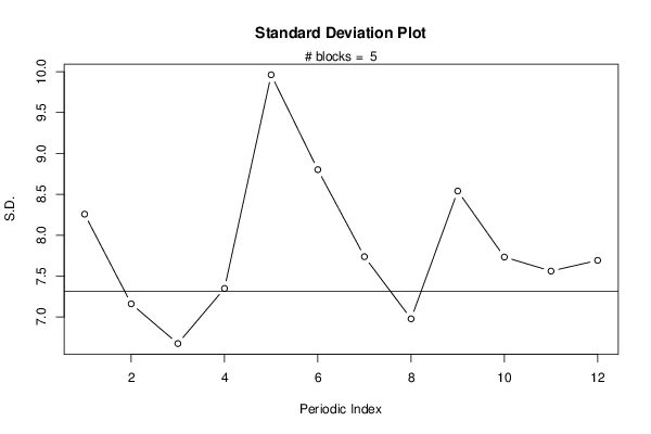
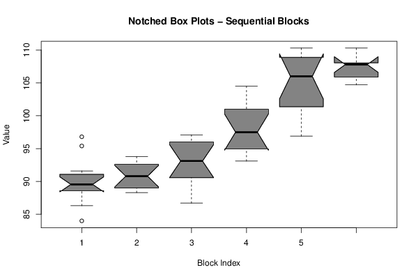
| Title produced by software | Standard Deviation Plot | ||||||||||||||||||||
| Date of computation | Tue, 22 Mar 2016 20:50:55 +0000 | ||||||||||||||||||||
| Cite this page as follows | Statistical Computations at FreeStatistics.org, Office for Research Development and Education, URL https://freestatistics.org/blog/index.php?v=date/2016/Mar/22/t145868002659y1txmgc677wkn.htm/, Retrieved Mon, 29 Apr 2024 09:37:45 +0000 | ||||||||||||||||||||
| Statistical Computations at FreeStatistics.org, Office for Research Development and Education, URL https://freestatistics.org/blog/index.php?pk=294481, Retrieved Mon, 29 Apr 2024 09:37:45 +0000 | |||||||||||||||||||||
| QR Codes: | |||||||||||||||||||||
|
| |||||||||||||||||||||
| Original text written by user: | |||||||||||||||||||||
| IsPrivate? | No (this computation is public) | ||||||||||||||||||||
| User-defined keywords | |||||||||||||||||||||
| Estimated Impact | 56 | ||||||||||||||||||||
Tree of Dependent Computations | |||||||||||||||||||||
| Family? (F = Feedback message, R = changed R code, M = changed R Module, P = changed Parameters, D = changed Data) | |||||||||||||||||||||
| - [Standard Deviation Plot] [] [2016-03-22 20:50:55] [66b954879edaa66f79d20403c5a86347] [Current] | |||||||||||||||||||||
| Feedback Forum | |||||||||||||||||||||
Post a new message | |||||||||||||||||||||
Dataset | |||||||||||||||||||||
| Dataseries X: | |||||||||||||||||||||
89,8 89,2 89,9 88,9 84 86,3 89,3 90,6 88,3 91,6 95,4 96,8 92,5 93,6 93,8 92,7 88,3 90,4 91,2 91,5 88,9 88,6 89,1 89,4 86,7 89,8 90,9 91,4 90,2 92,2 94 95,8 95,1 96,2 96,8 97,1 96,5 97,2 97,8 99,9 101,2 103,3 104,5 100,8 95 93,4 93,1 94,9 96,9 100,9 100,2 101,8 105,4 106,4 105,6 107,5 109,5 108,6 109,2 110,3 110,3 107,9 107,7 108,1 108 105,9 105,9 104,7 | |||||||||||||||||||||
Tables (Output of Computation) | |||||||||||||||||||||
| |||||||||||||||||||||
Figures (Output of Computation) | |||||||||||||||||||||
Input Parameters & R Code | |||||||||||||||||||||
| Parameters (Session): | |||||||||||||||||||||
| par1 = 12 ; | |||||||||||||||||||||
| Parameters (R input): | |||||||||||||||||||||
| par1 = 12 ; | |||||||||||||||||||||
| R code (references can be found in the software module): | |||||||||||||||||||||
par1 <- '12' | |||||||||||||||||||||