Repository of Reproducible Computations

Free Statistics

of Irreproducible Research!

Author's title

Author

*Unverified author*

R Software Module

rwasp_decompose.wasp

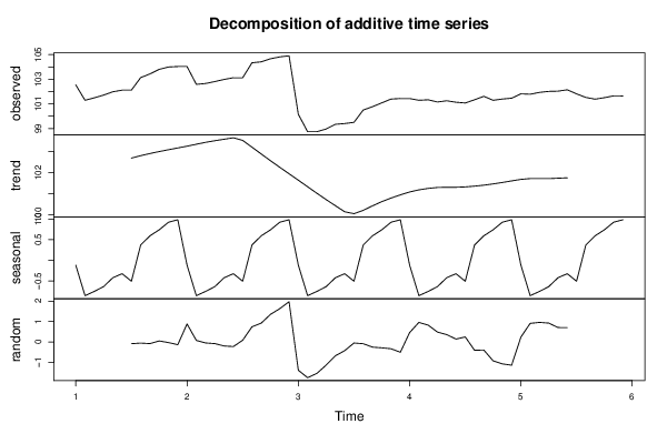
Title produced by software

Classical Decomposition

Date of computation

Sun, 27 Nov 2016 19:53:46 +0000

Cite this page as follows

Statistical Computations at FreeStatistics.org, Office for Research Development and Education, URL https://freestatistics.org/blog/index.php?v=date/2016/Nov/27/t1480276490r5f151zh6eqjm16.htm/, Retrieved Tue, 30 Apr 2024 01:50:21 +0200

Statistical Computations at FreeStatistics.org, Office for Research Development and Education, URL https://freestatistics.org/blog/index.php?pk=, Retrieved Tue, 30 Apr 2024 01:50:21 +0200

QR Codes:

Paste this QR Code to cite your computation.

Original text written by user:

IsPrivate?

No (this computation is public)

User-defined keywords

Estimated Impact

Dataseries X:

Download CSV

Histogram

Boxplots

Summary of computational transaction
Raw Input	view raw input (R code)
Raw Output	view raw output of R engine
Computing time	2 seconds
R Server	'Gertrude Mary Cox' @ cox.wessa.net

\begin{tabular}{lllllllll}
\hline
Summary of computational transaction \tabularnewline
Raw Input & view raw input (R code)  \tabularnewline
Raw Output & view raw output of R engine  \tabularnewline
Computing time & 2 seconds \tabularnewline
R Server & 'Gertrude Mary Cox' @ cox.wessa.net \tabularnewline
\hline
\end{tabular}
%Source: https://freestatistics.org/blog/index.php?pk=&T=0

[TABLE]
[ROW][C]Summary of computational transaction[/C][/ROW]
[ROW][C]Raw Input[/C][C]view raw input (R code) [/C][/ROW]
[ROW][C]Raw Output[/C][C]view raw output of R engine [/C][/ROW]
[ROW][C]Computing time[/C][C]2 seconds[/C][/ROW]
[ROW][C]R Server[/C][C]'Gertrude Mary Cox' @ cox.wessa.net[/C][/ROW]
[/TABLE]
Source: https://freestatistics.org/blog/index.php?pk=&T=0

Globally Unique Identifier (entire table): ba.freestatistics.org/blog/index.php?pk=&T=0

As an alternative you can also use a QR Code:

The GUIDs for individual cells are displayed in the table below:

Summary of computational transaction
Raw Input	view raw input (R code)
Raw Output	view raw output of R engine
Computing time	2 seconds
R Server	'Gertrude Mary Cox' @ cox.wessa.net

Classical Decomposition by Moving Averages
t	Observations	Fit	Trend	Seasonal	Random
1	102.54	NA	NA	-0.116311	NA
2	101.29	NA	NA	-0.853915	NA
3	101.49	NA	NA	-0.75079	NA
4	101.71	NA	NA	-0.635477	NA
5	101.98	NA	NA	-0.419644	NA
6	102.11	NA	NA	-0.322873	NA
7	102.11	102.192	102.696	-0.504748	-0.0815017
8	103.13	103.182	102.812	0.370252	-0.0523351
9	103.43	103.507	102.914	0.593064	-0.0772309
10	103.8	103.746	103.008	0.737856	0.0538108
11	103.99	104.018	103.096	0.92171	-0.0275434
12	104.03	104.16	103.18	0.980877	-0.13046
13	104.03	103.147	103.264	-0.116311	0.882561
14	102.58	102.502	103.356	-0.853915	0.0780816
15	102.65	102.696	103.447	-0.75079	-0.0458767
16	102.81	102.888	103.523	-0.635477	-0.0778559
17	102.98	103.174	103.593	-0.419644	-0.193689
18	103.12	103.341	103.664	-0.322873	-0.220877
19	103.12	103.034	103.538	-0.504748	0.0864149
20	104.33	103.587	103.217	0.370252	0.743082
21	104.41	103.487	102.894	0.593064	0.923186
22	104.66	103.308	102.57	0.737856	1.35173
23	104.81	103.18	102.258	0.92171	1.62996
24	104.9	102.933	101.952	0.980877	1.96746
25	100.15	101.53	101.646	-0.116311	-1.37952
26	98.74	100.482	101.335	-0.853915	-1.7415
27	98.74	100.273	101.024	-0.75079	-1.53338
28	98.96	100.088	100.723	-0.635477	-1.12786
29	99.34	100.012	100.432	-0.419644	-0.672023
30	99.4	99.8217	100.145	-0.322873	-0.42171
31	99.5	99.5486	100.053	-0.504748	-0.0485851
32	100.5	100.583	100.213	0.370252	-0.0831684
33	100.77	101.02	100.427	0.593064	-0.250148
34	101.08	101.364	100.626	0.737856	-0.284106
35	101.39	101.719	100.797	0.92171	-0.328793
36	101.43	101.93	100.949	0.980877	-0.499627
37	101.43	100.97	101.086	-0.116311	0.460061
38	101.29	100.332	101.186	-0.853915	0.957665
39	101.33	100.505	101.256	-0.75079	0.824957
40	101.15	100.664	101.3	-0.635477	0.485894
41	101.25	100.889	101.308	-0.419644	0.361311
42	101.13	100.987	101.31	-0.322873	0.14329
43	101.07	100.822	101.327	-0.504748	0.248082
44	101.33	101.733	101.363	0.370252	-0.403168
45	101.61	102.001	101.408	0.593064	-0.391398
46	101.29	102.207	101.469	0.737856	-0.917023
47	101.39	102.459	101.537	0.92171	-1.06921
48	101.46	102.593	101.612	0.980877	-1.13296
49	101.81	101.569	101.685	-0.116311	0.241311
50	101.78	100.87	101.724	-0.853915	0.910165
51	101.93	100.971	101.722	-0.75079	0.958707
52	102.01	101.086	101.721	-0.635477	0.924227
53	102.03	101.321	101.741	-0.419644	0.708811
54	102.14	101.436	101.759	-0.322873	0.703707
55	101.81	NA	NA	-0.504748	NA
56	101.52	NA	NA	0.370252	NA
57	101.38	NA	NA	0.593064	NA
58	101.5	NA	NA	0.737856	NA
59	101.65	NA	NA	0.92171	NA
60	101.64	NA	NA	0.980877	NA

\begin{tabular}{lllllllll}
\hline
Classical Decomposition by Moving Averages \tabularnewline
t & Observations & Fit & Trend & Seasonal & Random \tabularnewline
1 & 102.54 & NA & NA & -0.116311 & NA \tabularnewline
2 & 101.29 & NA & NA & -0.853915 & NA \tabularnewline
3 & 101.49 & NA & NA & -0.75079 & NA \tabularnewline
4 & 101.71 & NA & NA & -0.635477 & NA \tabularnewline
5 & 101.98 & NA & NA & -0.419644 & NA \tabularnewline
6 & 102.11 & NA & NA & -0.322873 & NA \tabularnewline
7 & 102.11 & 102.192 & 102.696 & -0.504748 & -0.0815017 \tabularnewline
8 & 103.13 & 103.182 & 102.812 & 0.370252 & -0.0523351 \tabularnewline
9 & 103.43 & 103.507 & 102.914 & 0.593064 & -0.0772309 \tabularnewline
10 & 103.8 & 103.746 & 103.008 & 0.737856 & 0.0538108 \tabularnewline
11 & 103.99 & 104.018 & 103.096 & 0.92171 & -0.0275434 \tabularnewline
12 & 104.03 & 104.16 & 103.18 & 0.980877 & -0.13046 \tabularnewline
13 & 104.03 & 103.147 & 103.264 & -0.116311 & 0.882561 \tabularnewline
14 & 102.58 & 102.502 & 103.356 & -0.853915 & 0.0780816 \tabularnewline
15 & 102.65 & 102.696 & 103.447 & -0.75079 & -0.0458767 \tabularnewline
16 & 102.81 & 102.888 & 103.523 & -0.635477 & -0.0778559 \tabularnewline
17 & 102.98 & 103.174 & 103.593 & -0.419644 & -0.193689 \tabularnewline
18 & 103.12 & 103.341 & 103.664 & -0.322873 & -0.220877 \tabularnewline
19 & 103.12 & 103.034 & 103.538 & -0.504748 & 0.0864149 \tabularnewline
20 & 104.33 & 103.587 & 103.217 & 0.370252 & 0.743082 \tabularnewline
21 & 104.41 & 103.487 & 102.894 & 0.593064 & 0.923186 \tabularnewline
22 & 104.66 & 103.308 & 102.57 & 0.737856 & 1.35173 \tabularnewline
23 & 104.81 & 103.18 & 102.258 & 0.92171 & 1.62996 \tabularnewline
24 & 104.9 & 102.933 & 101.952 & 0.980877 & 1.96746 \tabularnewline
25 & 100.15 & 101.53 & 101.646 & -0.116311 & -1.37952 \tabularnewline
26 & 98.74 & 100.482 & 101.335 & -0.853915 & -1.7415 \tabularnewline
27 & 98.74 & 100.273 & 101.024 & -0.75079 & -1.53338 \tabularnewline
28 & 98.96 & 100.088 & 100.723 & -0.635477 & -1.12786 \tabularnewline
29 & 99.34 & 100.012 & 100.432 & -0.419644 & -0.672023 \tabularnewline
30 & 99.4 & 99.8217 & 100.145 & -0.322873 & -0.42171 \tabularnewline
31 & 99.5 & 99.5486 & 100.053 & -0.504748 & -0.0485851 \tabularnewline
32 & 100.5 & 100.583 & 100.213 & 0.370252 & -0.0831684 \tabularnewline
33 & 100.77 & 101.02 & 100.427 & 0.593064 & -0.250148 \tabularnewline
34 & 101.08 & 101.364 & 100.626 & 0.737856 & -0.284106 \tabularnewline
35 & 101.39 & 101.719 & 100.797 & 0.92171 & -0.328793 \tabularnewline
36 & 101.43 & 101.93 & 100.949 & 0.980877 & -0.499627 \tabularnewline
37 & 101.43 & 100.97 & 101.086 & -0.116311 & 0.460061 \tabularnewline
38 & 101.29 & 100.332 & 101.186 & -0.853915 & 0.957665 \tabularnewline
39 & 101.33 & 100.505 & 101.256 & -0.75079 & 0.824957 \tabularnewline
40 & 101.15 & 100.664 & 101.3 & -0.635477 & 0.485894 \tabularnewline
41 & 101.25 & 100.889 & 101.308 & -0.419644 & 0.361311 \tabularnewline
42 & 101.13 & 100.987 & 101.31 & -0.322873 & 0.14329 \tabularnewline
43 & 101.07 & 100.822 & 101.327 & -0.504748 & 0.248082 \tabularnewline
44 & 101.33 & 101.733 & 101.363 & 0.370252 & -0.403168 \tabularnewline
45 & 101.61 & 102.001 & 101.408 & 0.593064 & -0.391398 \tabularnewline
46 & 101.29 & 102.207 & 101.469 & 0.737856 & -0.917023 \tabularnewline
47 & 101.39 & 102.459 & 101.537 & 0.92171 & -1.06921 \tabularnewline
48 & 101.46 & 102.593 & 101.612 & 0.980877 & -1.13296 \tabularnewline
49 & 101.81 & 101.569 & 101.685 & -0.116311 & 0.241311 \tabularnewline
50 & 101.78 & 100.87 & 101.724 & -0.853915 & 0.910165 \tabularnewline
51 & 101.93 & 100.971 & 101.722 & -0.75079 & 0.958707 \tabularnewline
52 & 102.01 & 101.086 & 101.721 & -0.635477 & 0.924227 \tabularnewline
53 & 102.03 & 101.321 & 101.741 & -0.419644 & 0.708811 \tabularnewline
54 & 102.14 & 101.436 & 101.759 & -0.322873 & 0.703707 \tabularnewline
55 & 101.81 & NA & NA & -0.504748 & NA \tabularnewline
56 & 101.52 & NA & NA & 0.370252 & NA \tabularnewline
57 & 101.38 & NA & NA & 0.593064 & NA \tabularnewline
58 & 101.5 & NA & NA & 0.737856 & NA \tabularnewline
59 & 101.65 & NA & NA & 0.92171 & NA \tabularnewline
60 & 101.64 & NA & NA & 0.980877 & NA \tabularnewline
\hline
\end{tabular}
%Source: https://freestatistics.org/blog/index.php?pk=&T=1

[TABLE]
[ROW][C]Classical Decomposition by Moving Averages[/C][/ROW]
[ROW][C]t[/C][C]Observations[/C][C]Fit[/C][C]Trend[/C][C]Seasonal[/C][C]Random[/C][/ROW]
[ROW][C]1[/C][C]102.54[/C][C]NA[/C][C]NA[/C][C]-0.116311[/C][C]NA[/C][/ROW]
[ROW][C]2[/C][C]101.29[/C][C]NA[/C][C]NA[/C][C]-0.853915[/C][C]NA[/C][/ROW]
[ROW][C]3[/C][C]101.49[/C][C]NA[/C][C]NA[/C][C]-0.75079[/C][C]NA[/C][/ROW]
[ROW][C]4[/C][C]101.71[/C][C]NA[/C][C]NA[/C][C]-0.635477[/C][C]NA[/C][/ROW]
[ROW][C]5[/C][C]101.98[/C][C]NA[/C][C]NA[/C][C]-0.419644[/C][C]NA[/C][/ROW]
[ROW][C]6[/C][C]102.11[/C][C]NA[/C][C]NA[/C][C]-0.322873[/C][C]NA[/C][/ROW]
[ROW][C]7[/C][C]102.11[/C][C]102.192[/C][C]102.696[/C][C]-0.504748[/C][C]-0.0815017[/C][/ROW]
[ROW][C]8[/C][C]103.13[/C][C]103.182[/C][C]102.812[/C][C]0.370252[/C][C]-0.0523351[/C][/ROW]
[ROW][C]9[/C][C]103.43[/C][C]103.507[/C][C]102.914[/C][C]0.593064[/C][C]-0.0772309[/C][/ROW]
[ROW][C]10[/C][C]103.8[/C][C]103.746[/C][C]103.008[/C][C]0.737856[/C][C]0.0538108[/C][/ROW]
[ROW][C]11[/C][C]103.99[/C][C]104.018[/C][C]103.096[/C][C]0.92171[/C][C]-0.0275434[/C][/ROW]
[ROW][C]12[/C][C]104.03[/C][C]104.16[/C][C]103.18[/C][C]0.980877[/C][C]-0.13046[/C][/ROW]
[ROW][C]13[/C][C]104.03[/C][C]103.147[/C][C]103.264[/C][C]-0.116311[/C][C]0.882561[/C][/ROW]
[ROW][C]14[/C][C]102.58[/C][C]102.502[/C][C]103.356[/C][C]-0.853915[/C][C]0.0780816[/C][/ROW]
[ROW][C]15[/C][C]102.65[/C][C]102.696[/C][C]103.447[/C][C]-0.75079[/C][C]-0.0458767[/C][/ROW]
[ROW][C]16[/C][C]102.81[/C][C]102.888[/C][C]103.523[/C][C]-0.635477[/C][C]-0.0778559[/C][/ROW]
[ROW][C]17[/C][C]102.98[/C][C]103.174[/C][C]103.593[/C][C]-0.419644[/C][C]-0.193689[/C][/ROW]
[ROW][C]18[/C][C]103.12[/C][C]103.341[/C][C]103.664[/C][C]-0.322873[/C][C]-0.220877[/C][/ROW]
[ROW][C]19[/C][C]103.12[/C][C]103.034[/C][C]103.538[/C][C]-0.504748[/C][C]0.0864149[/C][/ROW]
[ROW][C]20[/C][C]104.33[/C][C]103.587[/C][C]103.217[/C][C]0.370252[/C][C]0.743082[/C][/ROW]
[ROW][C]21[/C][C]104.41[/C][C]103.487[/C][C]102.894[/C][C]0.593064[/C][C]0.923186[/C][/ROW]
[ROW][C]22[/C][C]104.66[/C][C]103.308[/C][C]102.57[/C][C]0.737856[/C][C]1.35173[/C][/ROW]
[ROW][C]23[/C][C]104.81[/C][C]103.18[/C][C]102.258[/C][C]0.92171[/C][C]1.62996[/C][/ROW]
[ROW][C]24[/C][C]104.9[/C][C]102.933[/C][C]101.952[/C][C]0.980877[/C][C]1.96746[/C][/ROW]
[ROW][C]25[/C][C]100.15[/C][C]101.53[/C][C]101.646[/C][C]-0.116311[/C][C]-1.37952[/C][/ROW]
[ROW][C]26[/C][C]98.74[/C][C]100.482[/C][C]101.335[/C][C]-0.853915[/C][C]-1.7415[/C][/ROW]
[ROW][C]27[/C][C]98.74[/C][C]100.273[/C][C]101.024[/C][C]-0.75079[/C][C]-1.53338[/C][/ROW]
[ROW][C]28[/C][C]98.96[/C][C]100.088[/C][C]100.723[/C][C]-0.635477[/C][C]-1.12786[/C][/ROW]
[ROW][C]29[/C][C]99.34[/C][C]100.012[/C][C]100.432[/C][C]-0.419644[/C][C]-0.672023[/C][/ROW]
[ROW][C]30[/C][C]99.4[/C][C]99.8217[/C][C]100.145[/C][C]-0.322873[/C][C]-0.42171[/C][/ROW]
[ROW][C]31[/C][C]99.5[/C][C]99.5486[/C][C]100.053[/C][C]-0.504748[/C][C]-0.0485851[/C][/ROW]
[ROW][C]32[/C][C]100.5[/C][C]100.583[/C][C]100.213[/C][C]0.370252[/C][C]-0.0831684[/C][/ROW]
[ROW][C]33[/C][C]100.77[/C][C]101.02[/C][C]100.427[/C][C]0.593064[/C][C]-0.250148[/C][/ROW]
[ROW][C]34[/C][C]101.08[/C][C]101.364[/C][C]100.626[/C][C]0.737856[/C][C]-0.284106[/C][/ROW]
[ROW][C]35[/C][C]101.39[/C][C]101.719[/C][C]100.797[/C][C]0.92171[/C][C]-0.328793[/C][/ROW]
[ROW][C]36[/C][C]101.43[/C][C]101.93[/C][C]100.949[/C][C]0.980877[/C][C]-0.499627[/C][/ROW]
[ROW][C]37[/C][C]101.43[/C][C]100.97[/C][C]101.086[/C][C]-0.116311[/C][C]0.460061[/C][/ROW]
[ROW][C]38[/C][C]101.29[/C][C]100.332[/C][C]101.186[/C][C]-0.853915[/C][C]0.957665[/C][/ROW]
[ROW][C]39[/C][C]101.33[/C][C]100.505[/C][C]101.256[/C][C]-0.75079[/C][C]0.824957[/C][/ROW]
[ROW][C]40[/C][C]101.15[/C][C]100.664[/C][C]101.3[/C][C]-0.635477[/C][C]0.485894[/C][/ROW]
[ROW][C]41[/C][C]101.25[/C][C]100.889[/C][C]101.308[/C][C]-0.419644[/C][C]0.361311[/C][/ROW]
[ROW][C]42[/C][C]101.13[/C][C]100.987[/C][C]101.31[/C][C]-0.322873[/C][C]0.14329[/C][/ROW]
[ROW][C]43[/C][C]101.07[/C][C]100.822[/C][C]101.327[/C][C]-0.504748[/C][C]0.248082[/C][/ROW]
[ROW][C]44[/C][C]101.33[/C][C]101.733[/C][C]101.363[/C][C]0.370252[/C][C]-0.403168[/C][/ROW]
[ROW][C]45[/C][C]101.61[/C][C]102.001[/C][C]101.408[/C][C]0.593064[/C][C]-0.391398[/C][/ROW]
[ROW][C]46[/C][C]101.29[/C][C]102.207[/C][C]101.469[/C][C]0.737856[/C][C]-0.917023[/C][/ROW]
[ROW][C]47[/C][C]101.39[/C][C]102.459[/C][C]101.537[/C][C]0.92171[/C][C]-1.06921[/C][/ROW]
[ROW][C]48[/C][C]101.46[/C][C]102.593[/C][C]101.612[/C][C]0.980877[/C][C]-1.13296[/C][/ROW]
[ROW][C]49[/C][C]101.81[/C][C]101.569[/C][C]101.685[/C][C]-0.116311[/C][C]0.241311[/C][/ROW]
[ROW][C]50[/C][C]101.78[/C][C]100.87[/C][C]101.724[/C][C]-0.853915[/C][C]0.910165[/C][/ROW]
[ROW][C]51[/C][C]101.93[/C][C]100.971[/C][C]101.722[/C][C]-0.75079[/C][C]0.958707[/C][/ROW]
[ROW][C]52[/C][C]102.01[/C][C]101.086[/C][C]101.721[/C][C]-0.635477[/C][C]0.924227[/C][/ROW]
[ROW][C]53[/C][C]102.03[/C][C]101.321[/C][C]101.741[/C][C]-0.419644[/C][C]0.708811[/C][/ROW]
[ROW][C]54[/C][C]102.14[/C][C]101.436[/C][C]101.759[/C][C]-0.322873[/C][C]0.703707[/C][/ROW]
[ROW][C]55[/C][C]101.81[/C][C]NA[/C][C]NA[/C][C]-0.504748[/C][C]NA[/C][/ROW]
[ROW][C]56[/C][C]101.52[/C][C]NA[/C][C]NA[/C][C]0.370252[/C][C]NA[/C][/ROW]
[ROW][C]57[/C][C]101.38[/C][C]NA[/C][C]NA[/C][C]0.593064[/C][C]NA[/C][/ROW]
[ROW][C]58[/C][C]101.5[/C][C]NA[/C][C]NA[/C][C]0.737856[/C][C]NA[/C][/ROW]
[ROW][C]59[/C][C]101.65[/C][C]NA[/C][C]NA[/C][C]0.92171[/C][C]NA[/C][/ROW]
[ROW][C]60[/C][C]101.64[/C][C]NA[/C][C]NA[/C][C]0.980877[/C][C]NA[/C][/ROW]
[/TABLE]
Source: https://freestatistics.org/blog/index.php?pk=&T=1

Globally Unique Identifier (entire table): ba.freestatistics.org/blog/index.php?pk=&T=1

As an alternative you can also use a QR Code:

The GUIDs for individual cells are displayed in the table below:

Classical Decomposition by Moving Averages
t	Observations	Fit	Trend	Seasonal	Random
1	102.54	NA	NA	-0.116311	NA
2	101.29	NA	NA	-0.853915	NA
3	101.49	NA	NA	-0.75079	NA
4	101.71	NA	NA	-0.635477	NA
5	101.98	NA	NA	-0.419644	NA
6	102.11	NA	NA	-0.322873	NA
7	102.11	102.192	102.696	-0.504748	-0.0815017
8	103.13	103.182	102.812	0.370252	-0.0523351
9	103.43	103.507	102.914	0.593064	-0.0772309
10	103.8	103.746	103.008	0.737856	0.0538108
11	103.99	104.018	103.096	0.92171	-0.0275434
12	104.03	104.16	103.18	0.980877	-0.13046
13	104.03	103.147	103.264	-0.116311	0.882561
14	102.58	102.502	103.356	-0.853915	0.0780816
15	102.65	102.696	103.447	-0.75079	-0.0458767
16	102.81	102.888	103.523	-0.635477	-0.0778559
17	102.98	103.174	103.593	-0.419644	-0.193689
18	103.12	103.341	103.664	-0.322873	-0.220877
19	103.12	103.034	103.538	-0.504748	0.0864149
20	104.33	103.587	103.217	0.370252	0.743082
21	104.41	103.487	102.894	0.593064	0.923186
22	104.66	103.308	102.57	0.737856	1.35173
23	104.81	103.18	102.258	0.92171	1.62996
24	104.9	102.933	101.952	0.980877	1.96746
25	100.15	101.53	101.646	-0.116311	-1.37952
26	98.74	100.482	101.335	-0.853915	-1.7415
27	98.74	100.273	101.024	-0.75079	-1.53338
28	98.96	100.088	100.723	-0.635477	-1.12786
29	99.34	100.012	100.432	-0.419644	-0.672023
30	99.4	99.8217	100.145	-0.322873	-0.42171
31	99.5	99.5486	100.053	-0.504748	-0.0485851
32	100.5	100.583	100.213	0.370252	-0.0831684
33	100.77	101.02	100.427	0.593064	-0.250148
34	101.08	101.364	100.626	0.737856	-0.284106
35	101.39	101.719	100.797	0.92171	-0.328793
36	101.43	101.93	100.949	0.980877	-0.499627
37	101.43	100.97	101.086	-0.116311	0.460061
38	101.29	100.332	101.186	-0.853915	0.957665
39	101.33	100.505	101.256	-0.75079	0.824957
40	101.15	100.664	101.3	-0.635477	0.485894
41	101.25	100.889	101.308	-0.419644	0.361311
42	101.13	100.987	101.31	-0.322873	0.14329
43	101.07	100.822	101.327	-0.504748	0.248082
44	101.33	101.733	101.363	0.370252	-0.403168
45	101.61	102.001	101.408	0.593064	-0.391398
46	101.29	102.207	101.469	0.737856	-0.917023
47	101.39	102.459	101.537	0.92171	-1.06921
48	101.46	102.593	101.612	0.980877	-1.13296
49	101.81	101.569	101.685	-0.116311	0.241311
50	101.78	100.87	101.724	-0.853915	0.910165
51	101.93	100.971	101.722	-0.75079	0.958707
52	102.01	101.086	101.721	-0.635477	0.924227
53	102.03	101.321	101.741	-0.419644	0.708811
54	102.14	101.436	101.759	-0.322873	0.703707
55	101.81	NA	NA	-0.504748	NA
56	101.52	NA	NA	0.370252	NA
57	101.38	NA	NA	0.593064	NA
58	101.5	NA	NA	0.737856	NA
59	101.65	NA	NA	0.92171	NA
60	101.64	NA	NA	0.980877	NA

Figure 1

PNG link

Postscript link

PDF link

Figure 2

PNG link

Postscript link

PDF link

Figure 3

PNG link

Postscript link

PDF link

Figure 4

PNG link

Postscript link

PDF link

Parameters (Session):

par1 = additive ; par2 = 12 ;

Parameters (R input):

par1 = additive ; par2 = 12 ;

R code (references can be found in the software module):

par2 <- as.numeric(par2)
x <- ts(x,freq=par2)
m <- decompose(x,type=par1)
m$figure
bitmap(file='test1.png')
plot(m)
dev.off()
mylagmax <- length(x)/2
bitmap(file='test2.png')
op <- par(mfrow = c(2,2))
acf(as.numeric(x),lag.max = mylagmax,main='Observed')
acf(as.numeric(m$trend),na.action=na.pass,lag.max = mylagmax,main='Trend')
acf(as.numeric(m$seasonal),na.action=na.pass,lag.max = mylagmax,main='Seasonal')
acf(as.numeric(m$random),na.action=na.pass,lag.max = mylagmax,main='Random')
par(op)
dev.off()
bitmap(file='test3.png')
op <- par(mfrow = c(2,2))
spectrum(as.numeric(x),main='Observed')
spectrum(as.numeric(m$trend[!is.na(m$trend)]),main='Trend')
spectrum(as.numeric(m$seasonal[!is.na(m$seasonal)]),main='Seasonal')
spectrum(as.numeric(m$random[!is.na(m$random)]),main='Random')
par(op)
dev.off()
bitmap(file='test4.png')
op <- par(mfrow = c(2,2))
cpgram(as.numeric(x),main='Observed')
cpgram(as.numeric(m$trend[!is.na(m$trend)]),main='Trend')
cpgram(as.numeric(m$seasonal[!is.na(m$seasonal)]),main='Seasonal')
cpgram(as.numeric(m$random[!is.na(m$random)]),main='Random')
par(op)
dev.off()
load(file='createtable')
a<-table.start()
a<-table.row.start(a)
a<-table.element(a,'Classical Decomposition by Moving Averages',6,TRUE)
a<-table.row.end(a)
a<-table.row.start(a)
a<-table.element(a,'t',header=TRUE)
a<-table.element(a,'Observations',header=TRUE)
a<-table.element(a,'Fit',header=TRUE)
a<-table.element(a,'Trend',header=TRUE)
a<-table.element(a,'Seasonal',header=TRUE)
a<-table.element(a,'Random',header=TRUE)
a<-table.row.end(a)
for (i in 1:length(m$trend)) {
a<-table.row.start(a)
a<-table.element(a,i,header=TRUE)
a<-table.element(a,x[i])
if (par1 == 'additive') a<-table.element(a,signif(m$trend[i]+m$seasonal[i],6)) else a<-table.element(a,signif(m$trend[i]*m$seasonal[i],6))
a<-table.element(a,signif(m$trend[i],6))
a<-table.element(a,signif(m$seasonal[i],6))
a<-table.element(a,signif(m$random[i],6))
a<-table.row.end(a)
}
a<-table.end(a)
table.save(a,file='mytable.tab')

Free Statistics

Description of Statistical Computation

Tree of Dependent Computations

Dataset

Tables (Output of Computation)

Figures (Output of Computation)

Input Parameters & R Code