Repository of Reproducible Computations

Free Statistics

of Irreproducible Research!

Author's title

Author

*The author of this computation has been verified*

R Software Module

rwasp_fitdistrnorm.wasp

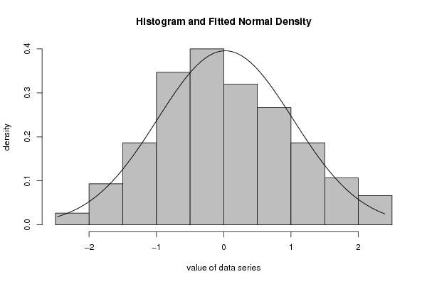
Title produced by software

ML Fitting and QQ Plot- Normal Distribution

Date of computation

Fri, 07 Oct 2016 14:03:45 +0200

Cite this page as follows

Statistical Computations at FreeStatistics.org, Office for Research Development and Education, URL https://freestatistics.org/blog/index.php?v=date/2016/Oct/07/t147584186472vlfsny9lxu8ca.htm/, Retrieved Mon, 06 May 2024 02:04:41 +0000

Statistical Computations at FreeStatistics.org, Office for Research Development and Education, URL https://freestatistics.org/blog/index.php?pk=296588, Retrieved Mon, 06 May 2024 02:04:41 +0000

QR Codes:

Paste this QR Code to cite your computation.

Original text written by user:

IsPrivate?

No (this computation is public)

User-defined keywords

Estimated Impact

Family? (F = Feedback message, R = changed R code, M = changed R Module, P = changed Parameters, D = changed Data)

-     [Binomial Probabilities] [bernoulli ] [2016-10-05 11:56:28] [2de65f32e81449e9ab36f33175b2d919]
- RMPD    [ML Fitting and QQ Plot- Normal Distribution] [3.3.7 -> problems...] [2016-10-07 12:03:45] [94ac3c9a028ddd47e8862e80eac9f626] [Current]

Feedback Forum

Post a new message

Dataseries X:

Download CSV

Histogram

Boxplots

-0.2342765522
-0.7081413518
0.3315939028
0.4190201728
-0.4712195263
-0.4037735785
-0.453029743
-0.5209788652
1.293037462
-1.656428005
0.5865280823
0.2253923446
2.011149497
1.128130737
-0.9996087018
0.3805541027
-0.2645973312
1.219849527
0.4332491497
-0.3206309813
1.603676636
1.858942724
-0.1474943889
1.655885625
0.8097810828
-0.9651774928
-1.239196012
-0.08554374132
0.5581677476
-1.250595277
0.3929261796
1.885230488
1.003017166
-1.235210483
-0.1029329017
-0.9359771283
1.17170111
-1.164683051
-0.4995157925
-0.2634432791
-0.1273812956
1.4239978
-1.340478259
0.1870816279
-0.4125908185
-0.09668101343
-0.8059897501
-0.6086329543
0.3475381883
-0.759575518
-0.5939588547
0.1940703001
0.5952599412
-0.8333292015
-0.8168842683
-1.029520193
0.02895408918
-1.168442248
2.085669891
-1.22736673
0.4328377008
-0.05896588016
-0.5810264421
-1.040189387
1.491052106
1.380178188
1.289404938
-0.686597505
-0.4138752266
0.3202536423
1.645100094
1.636153178
0.5818063385
-2.189860067
2.300977201
0.8357788287
-0.4097175693
0.8521382302
0.9481360577
-1.507039218
-1.276239393
-0.037847976
-0.8523675359
0.9137134063
0.8304323207
0.2142425372
0.3086275789
-0.3338724065
-0.7851902845
-0.2304403701
-0.3490873188
0.6014886387
1.342437677
0.8896474919
0.1518080129
-0.640230276
-2.471019422
1.434125212
-0.5225624207
-0.6405002406
-0.3863155591
1.842742422
-1.101621403
0.2720067133
-0.382786309
-0.398190071
-0.8103144424
0.980035775
0.3838630036
0.1950055674
0.5152900726
-1.979257455
0.2081441384
0.5385547059
-0.7032251437
-0.4869389877
-0.5542515044
-1.099214165
2.066523728
0.5694469773
1.108883065
-1.69393836
-1.694754679
-0.8080039466
0.4459831864
0.423083877
0.2638728713
0.6529369188
0.5057987289
-0.06242494444
0.7698388572
-1.640500702
-1.314143214
0.4093332172
0.01772387357
-0.7968425545
1.26529788
0.6136631181
-0.6557184497
2.393248047
-0.07791169145
-1.632818339
1.987837582
-0.2250366594
-0.7653930932
-0.1620012895
-1.167935656
-0.3682803654
1.167606986
-0.6597274473

Summary of computational transaction
Raw Input	view raw input (R code)
Raw Output	view raw output of R engine
Computing time	4 seconds
R Server	Big Analytics Cloud Computing Center

\begin{tabular}{lllllllll}
\hline
Summary of computational transaction \tabularnewline
Raw Input view raw input (R code)  \tabularnewline
Raw Outputview raw output of R engine  \tabularnewline
Computing time4 seconds \tabularnewline
R ServerBig Analytics Cloud Computing Center \tabularnewline
\hline
\end{tabular}
%Source: https://freestatistics.org/blog/index.php?pk=296588&T=0

[TABLE]
[ROW]

Summary of computational transaction[/C][/ROW] [ROW]

Raw Input[/C]

view raw input (R code) [/C][/ROW] [ROW]

Raw Output[/C]

view raw output of R engine [/C][/ROW] [ROW]

Computing time[/C]

4 seconds[/C][/ROW] [ROW]

R Server[/C]

Big Analytics Cloud Computing Center[/C][/ROW] [/TABLE] Source: https://freestatistics.org/blog/index.php?pk=296588&T=0

Globally Unique Identifier (entire table): ba.freestatistics.org/blog/index.php?pk=296588&T=0

As an alternative you can also use a QR Code:

The GUIDs for individual cells are displayed in the table below:

Summary of computational transaction
Raw Input	view raw input (R code)
Raw Output	view raw output of R engine
Computing time	4 seconds
R Server	Big Analytics Cloud Computing Center

Parameter	Estimated Value	Standard Deviation
mean	0.0228667040396667	0.0822867754321524
standard deviation	1.0078030619388	0.0581855369100496

\begin{tabular}{lllllllll}
\hline
Parameter & Estimated Value & Standard Deviation \tabularnewline
mean & 0.0228667040396667 & 0.0822867754321524 \tabularnewline
standard deviation & 1.0078030619388 & 0.0581855369100496 \tabularnewline
\hline
\end{tabular}
%Source: https://freestatistics.org/blog/index.php?pk=296588&T=1

[TABLE]
[ROW][C]Parameter[/C][C]Estimated Value[/C][C]Standard Deviation[/C][/ROW]
[ROW][C]mean[/C][C]0.0228667040396667[/C][C]0.0822867754321524[/C][/ROW]
[ROW][C]standard deviation[/C][C]1.0078030619388[/C][C]0.0581855369100496[/C][/ROW]
[/TABLE]
Source: https://freestatistics.org/blog/index.php?pk=296588&T=1

Globally Unique Identifier (entire table): ba.freestatistics.org/blog/index.php?pk=296588&T=1

As an alternative you can also use a QR Code:

The GUIDs for individual cells are displayed in the table below:

Parameter	Estimated Value	Standard Deviation
mean	0.0228667040396667	0.0822867754321524
standard deviation	1.0078030619388	0.0581855369100496

Figure 1

PNG link

Postscript link

PDF link

Figure 2

PNG link

Postscript link

PDF link

Parameters (Session):

par1 = 8 ; par2 = 0 ;

Parameters (R input):

par1 = 8 ; par2 = 0 ;

R code (references can be found in the software module):

library(MASS)
library(car)
par1 <- as.numeric(par1)
if (par2 == '0') par2 = 'Sturges' else par2 <- as.numeric(par2)
x <- as.ts(x) #otherwise the fitdistr function does not work properly
r <- fitdistr(x,'normal')
print(r)
bitmap(file='test1.png')
myhist<-hist(x,col=par1,breaks=par2,main=main,ylab=ylab,xlab=xlab,freq=F)
curve(1/(r$estimate[2]*sqrt(2*pi))*exp(-1/2*((x-r$estimate[1])/r$estimate[2])^2),min(x),max(x),add=T)
dev.off()
bitmap(file='test3.png')
qqPlot(x,dist='norm',main='QQ plot (Normal) with confidence intervals')
grid()
dev.off()
load(file='createtable')
a<-table.start()
a<-table.row.start(a)
a<-table.element(a,'Parameter',1,TRUE)
a<-table.element(a,'Estimated Value',1,TRUE)
a<-table.element(a,'Standard Deviation',1,TRUE)
a<-table.row.end(a)
a<-table.row.start(a)
a<-table.element(a,'mean',header=TRUE)
a<-table.element(a,r$estimate[1])
a<-table.element(a,r$sd[1])
a<-table.row.end(a)
a<-table.row.start(a)
a<-table.element(a,'standard deviation',header=TRUE)
a<-table.element(a,r$estimate[2])
a<-table.element(a,r$sd[2])
a<-table.row.end(a)
a<-table.end(a)
table.save(a,file='mytable.tab')

Free Statistics

Description of Statistical Computation

Tree of Dependent Computations

Dataset

Tables (Output of Computation)

Figures (Output of Computation)

Input Parameters & R Code