Free Statistics
of Irreproducible Research!
Description of Statistical Computation | ||||||||||||||||||||||||||||||||||||||||||||||||
|---|---|---|---|---|---|---|---|---|---|---|---|---|---|---|---|---|---|---|---|---|---|---|---|---|---|---|---|---|---|---|---|---|---|---|---|---|---|---|---|---|---|---|---|---|---|---|---|---|
| Author's title | ||||||||||||||||||||||||||||||||||||||||||||||||
| Author | *The author of this computation has been verified* | |||||||||||||||||||||||||||||||||||||||||||||||
| R Software Module | rwasp_fitdistrnorm.wasp | |||||||||||||||||||||||||||||||||||||||||||||||
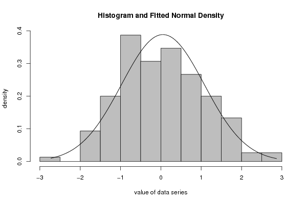
| Title produced by software | ML Fitting and QQ Plot- Normal Distribution | |||||||||||||||||||||||||||||||||||||||||||||||
| Date of computation | Fri, 07 Oct 2016 14:05:28 +0200 | |||||||||||||||||||||||||||||||||||||||||||||||
| Cite this page as follows | Statistical Computations at FreeStatistics.org, Office for Research Development and Education, URL https://freestatistics.org/blog/index.php?v=date/2016/Oct/07/t1475842185uldtigm9ff8dutq.htm/, Retrieved Sun, 05 May 2024 23:46:31 +0000 | |||||||||||||||||||||||||||||||||||||||||||||||
| Statistical Computations at FreeStatistics.org, Office for Research Development and Education, URL https://freestatistics.org/blog/index.php?pk=296593, Retrieved Sun, 05 May 2024 23:46:31 +0000 | ||||||||||||||||||||||||||||||||||||||||||||||||
| QR Codes: | ||||||||||||||||||||||||||||||||||||||||||||||||
|
| ||||||||||||||||||||||||||||||||||||||||||||||||
| Original text written by user: | ||||||||||||||||||||||||||||||||||||||||||||||||
| IsPrivate? | No (this computation is public) | |||||||||||||||||||||||||||||||||||||||||||||||
| User-defined keywords | ||||||||||||||||||||||||||||||||||||||||||||||||
| Estimated Impact | 115 | |||||||||||||||||||||||||||||||||||||||||||||||
Tree of Dependent Computations | ||||||||||||||||||||||||||||||||||||||||||||||||
| Family? (F = Feedback message, R = changed R code, M = changed R Module, P = changed Parameters, D = changed Data) | ||||||||||||||||||||||||||||||||||||||||||||||||
| - [ML Fitting and QQ Plot- Normal Distribution] [3.3.7.21.2 Kolom ...] [2016-10-07 12:05:28] [86c9a777e8dbb7ef3face68c75fc8376] [Current] | ||||||||||||||||||||||||||||||||||||||||||||||||
| Feedback Forum | ||||||||||||||||||||||||||||||||||||||||||||||||
Post a new message | ||||||||||||||||||||||||||||||||||||||||||||||||
Dataset | ||||||||||||||||||||||||||||||||||||||||||||||||
| Dataseries X: | ||||||||||||||||||||||||||||||||||||||||||||||||
-0.6469743537 0.09485047921 -1.518040426 -0.905984566 0.009199511133 0.167456977 -0.09025160405 0.5772186476 -0.559087047 -0.2556105576 1.278294177 -0.3323132719 0.4396190158 -1.049806751 -1.612960687 2.324874079 -1.301477848 -0.4305032655 -0.3010425348 -1.298417968 -0.5583932949 1.344007922 -0.5694807274 1.151893503 -0.5254599863 -0.8086130816 0.06353364996 1.160982486 2.657451193 1.34599268 -0.7211370029 -0.8032013496 -0.2004161904 -0.5784944392 1.31201442 0.4836270241 -0.02417507542 0.3954238657 -0.2693946272 -0.3024776894 0.2651077119 0.5154361624 0.6337046378 -0.4163812658 -0.08930972168 0.1276684164 -2.726952151 -0.5046855839 -1.097691244 -1.573194133 0.09612871307 1.855331085 0.9802057194 -0.8719097158 -0.7888354582 0.5386484994 0.06103339917 -0.9388080689 -0.7260629418 -0.822685846 0.08563205256 1.685956612 -1.203491474 -0.6128721473 -1.711316453 0.5300278621 1.877812151 -0.08379895612 -0.1097608908 -1.451656086 0.3561181945 0.7153917322 1.209123052 0.4045098004 -1.616625252 -1.0693862 0.198211182 0.6740444577 1.421423416 -0.1829782738 -0.5984163085 -1.030497192 -0.3399097364 0.5750699492 0.3335539653 -0.01252743344 0.8571516677 -0.8915521451 1.27957152 -1.522553199 -1.399825004 1.703888724 -0.4809993995 -0.8674294582 0.9902345562 1.632854909 0.9697731921 -0.5977367894 0.7475022968 -0.324902918 0.2549177519 0.2267152732 0.7387137971 1.564088846 0.1909621619 -0.3067390961 0.9265088912 -1.645663723 0.6982121744 0.6146243729 1.740647616 0.7105625806 1.132904828 -0.9709573063 2.871101073 -0.8812322455 0.04123668433 1.622262293 1.483017076 -0.980837159 0.3352670335 -0.9285885787 -0.1464389299 -0.1390202621 -1.109303571 1.310746789 1.430632039 -0.920844102 -1.433480031 0.7192761572 0.3134531805 -1.007106591 1.64655544 0.2302550199 0.1550377374 1.626094171 -1.297153221 -0.6374412712 0.486529959 1.449668944 -1.119057486 -0.8260702559 -0.5365791446 1.045722285 -0.3929513565 2.136099549 0.03363881635 -0.3063881621 -1.282942429 0.931785884 | ||||||||||||||||||||||||||||||||||||||||||||||||
Tables (Output of Computation) | ||||||||||||||||||||||||||||||||||||||||||||||||
| ||||||||||||||||||||||||||||||||||||||||||||||||
Figures (Output of Computation) | ||||||||||||||||||||||||||||||||||||||||||||||||
Input Parameters & R Code | ||||||||||||||||||||||||||||||||||||||||||||||||
| Parameters (Session): | ||||||||||||||||||||||||||||||||||||||||||||||||
| par1 = 8 ; par2 = 0 ; | ||||||||||||||||||||||||||||||||||||||||||||||||
| Parameters (R input): | ||||||||||||||||||||||||||||||||||||||||||||||||
| par1 = 8 ; par2 = 0 ; | ||||||||||||||||||||||||||||||||||||||||||||||||
| R code (references can be found in the software module): | ||||||||||||||||||||||||||||||||||||||||||||||||
library(MASS) | ||||||||||||||||||||||||||||||||||||||||||||||||