Repository of Reproducible Computations

Free Statistics

of Irreproducible Research!

Author's title

Author

*The author of this computation has been verified*

R Software Module

rwasp_fitdistrchisq1.wasp

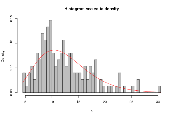
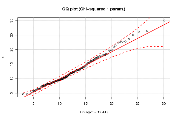
Title produced by software

Maximum-likelihood Fitting - Chi-squared Distribution

Date of computation

Fri, 07 Oct 2016 14:21:56 +0200

Cite this page as follows

Statistical Computations at FreeStatistics.org, Office for Research Development and Education, URL https://freestatistics.org/blog/index.php?v=date/2016/Oct/07/t1475843099scrmjrugjgkfl30.htm/, Retrieved Mon, 06 May 2024 07:01:49 +0000

Statistical Computations at FreeStatistics.org, Office for Research Development and Education, URL https://freestatistics.org/blog/index.php?pk=296603, Retrieved Mon, 06 May 2024 07:01:49 +0000

QR Codes:

Paste this QR Code to cite your computation.

Original text written by user:

IsPrivate?

No (this computation is public)

User-defined keywords

Estimated Impact

108

Family? (F = Feedback message, R = changed R code, M = changed R Module, P = changed Parameters, D = changed Data)

-     [Binomial Probabilities] [bernoulli ] [2016-10-05 11:56:28] [2de65f32e81449e9ab36f33175b2d919]
- RMPD    [Maximum-likelihood Fitting - Chi-squared Distribution] [3.3.7 -> problems...] [2016-10-07 12:21:56] [94ac3c9a028ddd47e8862e80eac9f626] [Current]

Feedback Forum

Post a new message

Dataseries X:

Download CSV

Histogram

Boxplots

19.39462165
11.96993472
5.658953516
9.408410443
12.12154573
13.8659245
9.627530481
11.02351026
8.53023382
17.83591
11.43980066
12.4030446
8.097939877
7.464382648
9.98878218
13.92281255
18.14877509
9.541609389
9.239468407
8.286216455
9.126216225
4.630766748
12.83771582
7.941657957
12.37892879
13.31122082
14.89255434
18.45772281
10.28060747
7.952892215
11.67276947
8.95347598
9.414047453
16.55778777
11.39413811
22.24307364
8.260192629
13.56603098
13.69656614
22.6572334
11.8395421
9.975467977
17.64373438
13.46071253
13.00911438
9.815307699
9.330068507
12.48079304
8.151022796
12.90684876
9.726076576
9.116861598
4.733537741
26.45228515
16.00708061
15.38094513
15.54786829
30.00327564
10.10592033
21.41135157
12.40594328
10.15370284
8.396111968
7.386007057
6.47562133
6.547877884
8.163491362
12.49860712
12.94144981
15.99571337
4.651328832
5.481473454
8.834860472
16.2242812
6.4384344
12.25857833
11.78764945
5.814828436
10.68399287
10.38173217
14.83102783
8.962375542
18.17045991
9.045837089
9.858964701
12.20663495
9.847077972
16.16823692
14.21272961
22.77201977
9.541135452
17.45293384
15.38486601
23.54648779
10.71826767
10.5203
20.92015393
13.86067593
18.11539442
13.11878651
10.18515358
11.10297417
17.33378461
7.601425014
8.605525971
7.351236431
7.36284027
8.181667065
8.686406736
7.262184518
9.393969933
17.81001553
11.36599643
11.90197003
19.4437225
17.05470486
6.112584193
26.18455144
9.100594106
5.636372782
16.81433166
19.97440111
14.20970782
9.604065162
18.49076841
11.96044229
8.688725333
14.28795299
7.989856641
7.59797464
12.79887061
14.87778575
13.09442835
15.29263502
25.01938851
10.49918073
8.149225429
7.289823029
10.91314457
6.568555623
16.35499606
17.05397068
9.928866966
13.05317762
13.51892274
6.299855411
22.71365352
9.49459111
8.912206471
8.258283799

Summary of computational transaction
Raw Input	view raw input (R code)
Raw Output	view raw output of R engine
Computing time	4 seconds
R Server	Big Analytics Cloud Computing Center

\begin{tabular}{lllllllll}
\hline
Summary of computational transaction \tabularnewline
Raw Input view raw input (R code)  \tabularnewline
Raw Outputview raw output of R engine  \tabularnewline
Computing time4 seconds \tabularnewline
R ServerBig Analytics Cloud Computing Center \tabularnewline
\hline
\end{tabular}
%Source: https://freestatistics.org/blog/index.php?pk=296603&T=0

[TABLE]
[ROW]

Summary of computational transaction[/C][/ROW] [ROW]

Raw Input[/C]

view raw input (R code) [/C][/ROW] [ROW]

Raw Output[/C]

view raw output of R engine [/C][/ROW] [ROW]

Computing time[/C]

4 seconds[/C][/ROW] [ROW]

R Server[/C]

Big Analytics Cloud Computing Center[/C][/ROW] [/TABLE] Source: https://freestatistics.org/blog/index.php?pk=296603&T=0

Globally Unique Identifier (entire table): ba.freestatistics.org/blog/index.php?pk=296603&T=0

As an alternative you can also use a QR Code:

The GUIDs for individual cells are displayed in the table below:

Summary of computational transaction
Raw Input	view raw input (R code)
Raw Output	view raw output of R engine
Computing time	4 seconds
R Server	Big Analytics Cloud Computing Center

Parameter	Estimated Value	Standard Deviation
df	12.4146435150419	0.390616821663621

\begin{tabular}{lllllllll}
\hline
Parameter & Estimated Value & Standard Deviation \tabularnewline
df & 12.4146435150419 & 0.390616821663621 \tabularnewline
\hline
\end{tabular}
%Source: https://freestatistics.org/blog/index.php?pk=296603&T=1

[TABLE]
[ROW][C]Parameter[/C][C]Estimated Value[/C][C]Standard Deviation[/C][/ROW]
[ROW][C]df[/C][C]12.4146435150419[/C][C]0.390616821663621[/C][/ROW]
[/TABLE]
Source: https://freestatistics.org/blog/index.php?pk=296603&T=1

Globally Unique Identifier (entire table): ba.freestatistics.org/blog/index.php?pk=296603&T=1

As an alternative you can also use a QR Code:

The GUIDs for individual cells are displayed in the table below:

Parameter	Estimated Value	Standard Deviation
df	12.4146435150419	0.390616821663621

Figure 1

PNG link

Postscript link

PDF link

Figure 2

PNG link

Postscript link

PDF link

Parameters (Session):

par1 = 8 ; par2 = 0 ;

Parameters (R input):

R code (references can be found in the software module):

library(MASS)
library(car)
chii <- x
chi_df <- fitdistr(chii,'chi-squared',start=list(df=3), method='Brent',lower=0.1,upper=100)
chi_k <- chi_df[[1]][1]
bitmap(file='test1.png')
chi_hist <- hist(chii,breaks=50,col='gray',freq=FALSE,main='Histogram scaled to density',xlab='x')
curve(dchisq(x,df=chi_k),add=TRUE,col='red')
dev.off()
f<-chi_df
f$estimate
f$sd
xlab <- paste('Chisq(df = ',round(f$estimate[[1]],2),sep='')
xlab <- paste(xlab,')',sep='')
xlab
bitmap(file='test2.png')
qqPlot(x, dist='chisq', df=f$estimate[[1]], ncp=0, main='QQ plot (Chi-squared 1 param.)', xlab=xlab )
grid()
dev.off()
load(file='createtable')
a<-table.start()
a<-table.row.start(a)
a<-table.element(a,'Parameter',1,TRUE)
a<-table.element(a,'Estimated Value',1,TRUE)
a<-table.element(a,'Standard Deviation',1,TRUE)
a<-table.row.end(a)
a<-table.row.start(a)
a<-table.element(a,'df',header=TRUE)
a<-table.element(a,f$estimate[1])
a<-table.element(a,f$sd[1])
a<-table.row.end(a)
a<-table.end(a)
table.save(a,file='mytable.tab')

Free Statistics

Description of Statistical Computation

Tree of Dependent Computations

Dataset

Tables (Output of Computation)

Figures (Output of Computation)

Input Parameters & R Code