Repository of Reproducible Computations

Free Statistics

of Irreproducible Research!

Author's title

Author

*Unverified author*

R Software Module

rwasp_autocorrelation.wasp

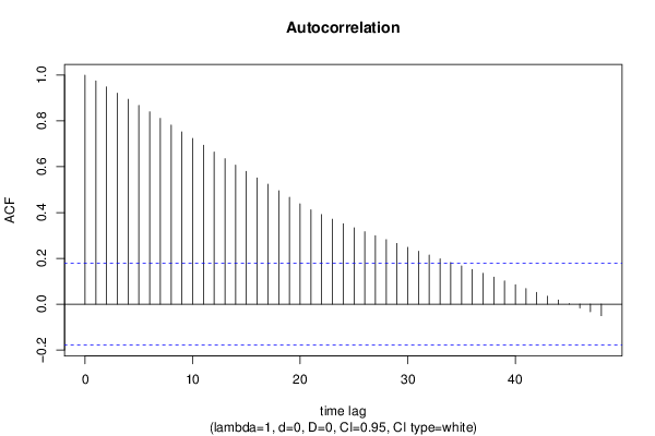
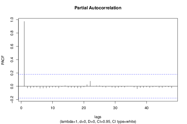
Title produced by software

(Partial) Autocorrelation Function

Date of computation

Tue, 18 Oct 2016 15:52:01 +0100

Cite this page as follows

Statistical Computations at FreeStatistics.org, Office for Research Development and Education, URL https://freestatistics.org/blog/index.php?v=date/2016/Oct/18/t1476802373pmqwkgd4ip8pc9w.htm/, Retrieved Sun, 28 Apr 2024 02:24:20 +0200

Statistical Computations at FreeStatistics.org, Office for Research Development and Education, URL https://freestatistics.org/blog/index.php?pk=, Retrieved Sun, 28 Apr 2024 02:24:20 +0200

QR Codes:

Paste this QR Code to cite your computation.

Original text written by user:

IsPrivate?

No (this computation is public)

User-defined keywords

Estimated Impact

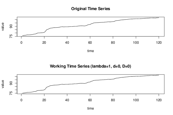
Dataseries X:

Download CSV

Histogram

Boxplots

Summary of computational transaction
Raw Input	view raw input (R code)
Raw Output	view raw output of R engine
Computing time	2 seconds
R Server	'Gwilym Jenkins' @ jenkins.wessa.net

\begin{tabular}{lllllllll}
\hline
Summary of computational transaction \tabularnewline
Raw Input & view raw input (R code)  \tabularnewline
Raw Output & view raw output of R engine  \tabularnewline
Computing time & 2 seconds \tabularnewline
R Server & 'Gwilym Jenkins' @ jenkins.wessa.net \tabularnewline
\hline
\end{tabular}
%Source: https://freestatistics.org/blog/index.php?pk=&T=0

[TABLE]
[ROW][C]Summary of computational transaction[/C][/ROW]
[ROW][C]Raw Input[/C][C]view raw input (R code) [/C][/ROW]
[ROW][C]Raw Output[/C][C]view raw output of R engine [/C][/ROW]
[ROW][C]Computing time[/C][C]2 seconds[/C][/ROW]
[ROW][C]R Server[/C][C]'Gwilym Jenkins' @ jenkins.wessa.net[/C][/ROW]
[/TABLE]
Source: https://freestatistics.org/blog/index.php?pk=&T=0

Globally Unique Identifier (entire table): ba.freestatistics.org/blog/index.php?pk=&T=0

As an alternative you can also use a QR Code:

The GUIDs for individual cells are displayed in the table below:

Summary of computational transaction
Raw Input	view raw input (R code)
Raw Output	view raw output of R engine
Computing time	2 seconds
R Server	'Gwilym Jenkins' @ jenkins.wessa.net

Autocorrelation Function
Time lag k	ACF(k)	T-STAT	P-value
1	0.974558	10.6757	0
2	0.948423	10.3895	0
3	0.921603	10.0957	0
4	0.894626	9.8001	0
5	0.867597	9.5041	0
6	0.83976	9.1991	0
7	0.811273	8.887	0
8	0.782178	8.5683	0
9	0.752739	8.2458	0
10	0.723394	7.9244	0
11	0.694166	7.6042	0
12	0.664462	7.2788	0
13	0.63525	6.9588	0
14	0.607355	6.6532	0
15	0.579489	6.348	0
16	0.551614	6.0426	0
17	0.523664	5.7365	0
18	0.495332	5.4261	0
19	0.466668	5.1121	1e-06
20	0.438425	4.8027	2e-06
21	0.412399	4.5176	7e-06
22	0.391206	4.2854	1.9e-05
23	0.370831	4.0622	4.4e-05
24	0.351723	3.8529	9.4e-05
25	0.333849	3.6571	0.00019
26	0.316246	3.4643	0.000369
27	0.298694	3.272	0.000697
28	0.281892	3.088	0.001252
29	0.265214	2.9053	0.002185
30	0.248259	2.7195	0.003754
31	0.231211	2.5328	0.006303
32	0.2145	2.3497	0.01021
33	0.197861	2.1675	0.016088
34	0.181883	1.9924	0.024297
35	0.166519	1.8241	0.035311
36	0.151186	1.6562	0.050151
37	0.134688	1.4754	0.071358
38	0.117947	1.292	0.099412
39	0.101231	1.1089	0.134838
40	0.084914	0.9302	0.177071
41	0.068331	0.7485	0.227804
42	0.051651	0.5658	0.28629
43	0.035034	0.3838	0.350911
44	0.018109	0.1984	0.421542
45	0.000767	0.0084	0.496655
46	-0.016295	-0.1785	0.429313
47	-0.033148	-0.3631	0.358576
48	-0.050414	-0.5523	0.2909

\begin{tabular}{lllllllll}
\hline
Autocorrelation Function \tabularnewline
Time lag k & ACF(k) & T-STAT & P-value \tabularnewline
1 & 0.974558 & 10.6757 & 0 \tabularnewline
2 & 0.948423 & 10.3895 & 0 \tabularnewline
3 & 0.921603 & 10.0957 & 0 \tabularnewline
4 & 0.894626 & 9.8001 & 0 \tabularnewline
5 & 0.867597 & 9.5041 & 0 \tabularnewline
6 & 0.83976 & 9.1991 & 0 \tabularnewline
7 & 0.811273 & 8.887 & 0 \tabularnewline
8 & 0.782178 & 8.5683 & 0 \tabularnewline
9 & 0.752739 & 8.2458 & 0 \tabularnewline
10 & 0.723394 & 7.9244 & 0 \tabularnewline
11 & 0.694166 & 7.6042 & 0 \tabularnewline
12 & 0.664462 & 7.2788 & 0 \tabularnewline
13 & 0.63525 & 6.9588 & 0 \tabularnewline
14 & 0.607355 & 6.6532 & 0 \tabularnewline
15 & 0.579489 & 6.348 & 0 \tabularnewline
16 & 0.551614 & 6.0426 & 0 \tabularnewline
17 & 0.523664 & 5.7365 & 0 \tabularnewline
18 & 0.495332 & 5.4261 & 0 \tabularnewline
19 & 0.466668 & 5.1121 & 1e-06 \tabularnewline
20 & 0.438425 & 4.8027 & 2e-06 \tabularnewline
21 & 0.412399 & 4.5176 & 7e-06 \tabularnewline
22 & 0.391206 & 4.2854 & 1.9e-05 \tabularnewline
23 & 0.370831 & 4.0622 & 4.4e-05 \tabularnewline
24 & 0.351723 & 3.8529 & 9.4e-05 \tabularnewline
25 & 0.333849 & 3.6571 & 0.00019 \tabularnewline
26 & 0.316246 & 3.4643 & 0.000369 \tabularnewline
27 & 0.298694 & 3.272 & 0.000697 \tabularnewline
28 & 0.281892 & 3.088 & 0.001252 \tabularnewline
29 & 0.265214 & 2.9053 & 0.002185 \tabularnewline
30 & 0.248259 & 2.7195 & 0.003754 \tabularnewline
31 & 0.231211 & 2.5328 & 0.006303 \tabularnewline
32 & 0.2145 & 2.3497 & 0.01021 \tabularnewline
33 & 0.197861 & 2.1675 & 0.016088 \tabularnewline
34 & 0.181883 & 1.9924 & 0.024297 \tabularnewline
35 & 0.166519 & 1.8241 & 0.035311 \tabularnewline
36 & 0.151186 & 1.6562 & 0.050151 \tabularnewline
37 & 0.134688 & 1.4754 & 0.071358 \tabularnewline
38 & 0.117947 & 1.292 & 0.099412 \tabularnewline
39 & 0.101231 & 1.1089 & 0.134838 \tabularnewline
40 & 0.084914 & 0.9302 & 0.177071 \tabularnewline
41 & 0.068331 & 0.7485 & 0.227804 \tabularnewline
42 & 0.051651 & 0.5658 & 0.28629 \tabularnewline
43 & 0.035034 & 0.3838 & 0.350911 \tabularnewline
44 & 0.018109 & 0.1984 & 0.421542 \tabularnewline
45 & 0.000767 & 0.0084 & 0.496655 \tabularnewline
46 & -0.016295 & -0.1785 & 0.429313 \tabularnewline
47 & -0.033148 & -0.3631 & 0.358576 \tabularnewline
48 & -0.050414 & -0.5523 & 0.2909 \tabularnewline
\hline
\end{tabular}
%Source: https://freestatistics.org/blog/index.php?pk=&T=1

[TABLE]
[ROW][C]Autocorrelation Function[/C][/ROW]
[ROW][C]Time lag k[/C][C]ACF(k)[/C][C]T-STAT[/C][C]P-value[/C][/ROW]
[ROW][C]1[/C][C]0.974558[/C][C]10.6757[/C][C]0[/C][/ROW]
[ROW][C]2[/C][C]0.948423[/C][C]10.3895[/C][C]0[/C][/ROW]
[ROW][C]3[/C][C]0.921603[/C][C]10.0957[/C][C]0[/C][/ROW]
[ROW][C]4[/C][C]0.894626[/C][C]9.8001[/C][C]0[/C][/ROW]
[ROW][C]5[/C][C]0.867597[/C][C]9.5041[/C][C]0[/C][/ROW]
[ROW][C]6[/C][C]0.83976[/C][C]9.1991[/C][C]0[/C][/ROW]
[ROW][C]7[/C][C]0.811273[/C][C]8.887[/C][C]0[/C][/ROW]
[ROW][C]8[/C][C]0.782178[/C][C]8.5683[/C][C]0[/C][/ROW]
[ROW][C]9[/C][C]0.752739[/C][C]8.2458[/C][C]0[/C][/ROW]
[ROW][C]10[/C][C]0.723394[/C][C]7.9244[/C][C]0[/C][/ROW]
[ROW][C]11[/C][C]0.694166[/C][C]7.6042[/C][C]0[/C][/ROW]
[ROW][C]12[/C][C]0.664462[/C][C]7.2788[/C][C]0[/C][/ROW]
[ROW][C]13[/C][C]0.63525[/C][C]6.9588[/C][C]0[/C][/ROW]
[ROW][C]14[/C][C]0.607355[/C][C]6.6532[/C][C]0[/C][/ROW]
[ROW][C]15[/C][C]0.579489[/C][C]6.348[/C][C]0[/C][/ROW]
[ROW][C]16[/C][C]0.551614[/C][C]6.0426[/C][C]0[/C][/ROW]
[ROW][C]17[/C][C]0.523664[/C][C]5.7365[/C][C]0[/C][/ROW]
[ROW][C]18[/C][C]0.495332[/C][C]5.4261[/C][C]0[/C][/ROW]
[ROW][C]19[/C][C]0.466668[/C][C]5.1121[/C][C]1e-06[/C][/ROW]
[ROW][C]20[/C][C]0.438425[/C][C]4.8027[/C][C]2e-06[/C][/ROW]
[ROW][C]21[/C][C]0.412399[/C][C]4.5176[/C][C]7e-06[/C][/ROW]
[ROW][C]22[/C][C]0.391206[/C][C]4.2854[/C][C]1.9e-05[/C][/ROW]
[ROW][C]23[/C][C]0.370831[/C][C]4.0622[/C][C]4.4e-05[/C][/ROW]
[ROW][C]24[/C][C]0.351723[/C][C]3.8529[/C][C]9.4e-05[/C][/ROW]
[ROW][C]25[/C][C]0.333849[/C][C]3.6571[/C][C]0.00019[/C][/ROW]
[ROW][C]26[/C][C]0.316246[/C][C]3.4643[/C][C]0.000369[/C][/ROW]
[ROW][C]27[/C][C]0.298694[/C][C]3.272[/C][C]0.000697[/C][/ROW]
[ROW][C]28[/C][C]0.281892[/C][C]3.088[/C][C]0.001252[/C][/ROW]
[ROW][C]29[/C][C]0.265214[/C][C]2.9053[/C][C]0.002185[/C][/ROW]
[ROW][C]30[/C][C]0.248259[/C][C]2.7195[/C][C]0.003754[/C][/ROW]
[ROW][C]31[/C][C]0.231211[/C][C]2.5328[/C][C]0.006303[/C][/ROW]
[ROW][C]32[/C][C]0.2145[/C][C]2.3497[/C][C]0.01021[/C][/ROW]
[ROW][C]33[/C][C]0.197861[/C][C]2.1675[/C][C]0.016088[/C][/ROW]
[ROW][C]34[/C][C]0.181883[/C][C]1.9924[/C][C]0.024297[/C][/ROW]
[ROW][C]35[/C][C]0.166519[/C][C]1.8241[/C][C]0.035311[/C][/ROW]
[ROW][C]36[/C][C]0.151186[/C][C]1.6562[/C][C]0.050151[/C][/ROW]
[ROW][C]37[/C][C]0.134688[/C][C]1.4754[/C][C]0.071358[/C][/ROW]
[ROW][C]38[/C][C]0.117947[/C][C]1.292[/C][C]0.099412[/C][/ROW]
[ROW][C]39[/C][C]0.101231[/C][C]1.1089[/C][C]0.134838[/C][/ROW]
[ROW][C]40[/C][C]0.084914[/C][C]0.9302[/C][C]0.177071[/C][/ROW]
[ROW][C]41[/C][C]0.068331[/C][C]0.7485[/C][C]0.227804[/C][/ROW]
[ROW][C]42[/C][C]0.051651[/C][C]0.5658[/C][C]0.28629[/C][/ROW]
[ROW][C]43[/C][C]0.035034[/C][C]0.3838[/C][C]0.350911[/C][/ROW]
[ROW][C]44[/C][C]0.018109[/C][C]0.1984[/C][C]0.421542[/C][/ROW]
[ROW][C]45[/C][C]0.000767[/C][C]0.0084[/C][C]0.496655[/C][/ROW]
[ROW][C]46[/C][C]-0.016295[/C][C]-0.1785[/C][C]0.429313[/C][/ROW]
[ROW][C]47[/C][C]-0.033148[/C][C]-0.3631[/C][C]0.358576[/C][/ROW]
[ROW][C]48[/C][C]-0.050414[/C][C]-0.5523[/C][C]0.2909[/C][/ROW]
[/TABLE]
Source: https://freestatistics.org/blog/index.php?pk=&T=1

Globally Unique Identifier (entire table): ba.freestatistics.org/blog/index.php?pk=&T=1

As an alternative you can also use a QR Code:

The GUIDs for individual cells are displayed in the table below:

Autocorrelation Function
Time lag k	ACF(k)	T-STAT	P-value
1	0.974558	10.6757	0
2	0.948423	10.3895	0
3	0.921603	10.0957	0
4	0.894626	9.8001	0
5	0.867597	9.5041	0
6	0.83976	9.1991	0
7	0.811273	8.887	0
8	0.782178	8.5683	0
9	0.752739	8.2458	0
10	0.723394	7.9244	0
11	0.694166	7.6042	0
12	0.664462	7.2788	0
13	0.63525	6.9588	0
14	0.607355	6.6532	0
15	0.579489	6.348	0
16	0.551614	6.0426	0
17	0.523664	5.7365	0
18	0.495332	5.4261	0
19	0.466668	5.1121	1e-06
20	0.438425	4.8027	2e-06
21	0.412399	4.5176	7e-06
22	0.391206	4.2854	1.9e-05
23	0.370831	4.0622	4.4e-05
24	0.351723	3.8529	9.4e-05
25	0.333849	3.6571	0.00019
26	0.316246	3.4643	0.000369
27	0.298694	3.272	0.000697
28	0.281892	3.088	0.001252
29	0.265214	2.9053	0.002185
30	0.248259	2.7195	0.003754
31	0.231211	2.5328	0.006303
32	0.2145	2.3497	0.01021
33	0.197861	2.1675	0.016088
34	0.181883	1.9924	0.024297
35	0.166519	1.8241	0.035311
36	0.151186	1.6562	0.050151
37	0.134688	1.4754	0.071358
38	0.117947	1.292	0.099412
39	0.101231	1.1089	0.134838
40	0.084914	0.9302	0.177071
41	0.068331	0.7485	0.227804
42	0.051651	0.5658	0.28629
43	0.035034	0.3838	0.350911
44	0.018109	0.1984	0.421542
45	0.000767	0.0084	0.496655
46	-0.016295	-0.1785	0.429313
47	-0.033148	-0.3631	0.358576
48	-0.050414	-0.5523	0.2909

Partial Autocorrelation Function
Time lag k	PACF(k)	T-STAT	P-value
1	0.974558	10.6757	0
2	-0.026674	-0.2922	0.385319
3	-0.026864	-0.2943	0.384528
4	-0.016757	-0.1836	0.427334
5	-0.015008	-0.1644	0.434843
6	-0.030494	-0.334	0.369463
7	-0.027693	-0.3034	0.381071
8	-0.027154	-0.2975	0.383314
9	-0.022538	-0.2469	0.402706
10	-0.01447	-0.1585	0.43716
11	-0.014293	-0.1566	0.437921
12	-0.02652	-0.2905	0.385963
13	-0.007378	-0.0808	0.467857
14	0.008964	0.0982	0.460969
15	-0.017345	-0.19	0.424813
16	-0.01849	-0.2025	0.419917
17	-0.019332	-0.2118	0.416323
18	-0.026088	-0.2858	0.387769
19	-0.026239	-0.2874	0.387139
20	-0.011485	-0.1258	0.450044
21	0.024089	0.2639	0.39616
22	0.077143	0.8451	0.199881
23	-0.001628	-0.0178	0.492899
24	0.007709	0.0845	0.466419
25	0.008415	0.0922	0.463352
26	-0.010884	-0.1192	0.452648
27	-0.017789	-0.1949	0.422911
28	-0.00389	-0.0426	0.483038
29	-0.016121	-0.1766	0.430061
30	-0.023449	-0.2569	0.398859
31	-0.018667	-0.2045	0.419158
32	-0.010074	-0.1104	0.456156
33	-0.015398	-0.1687	0.433166
34	0.001027	0.0113	0.49552
35	0.001418	0.0155	0.493816
36	-0.014502	-0.1589	0.437023
37	-0.038453	-0.4212	0.337171
38	-0.021337	-0.2337	0.407795
39	-0.019161	-0.2099	0.417052
40	-0.011422	-0.1251	0.450318
41	-0.020522	-0.2248	0.411258
42	-0.012154	-0.1331	0.447154
43	-0.006401	-0.0701	0.472108
44	-0.018481	-0.2025	0.419952
45	-0.019905	-0.2181	0.41388
46	-0.007443	-0.0815	0.467577
47	-0.011366	-0.1245	0.450563
48	-0.024309	-0.2663	0.395237

\begin{tabular}{lllllllll}
\hline
Partial Autocorrelation Function \tabularnewline
Time lag k & PACF(k) & T-STAT & P-value \tabularnewline
1 & 0.974558 & 10.6757 & 0 \tabularnewline
2 & -0.026674 & -0.2922 & 0.385319 \tabularnewline
3 & -0.026864 & -0.2943 & 0.384528 \tabularnewline
4 & -0.016757 & -0.1836 & 0.427334 \tabularnewline
5 & -0.015008 & -0.1644 & 0.434843 \tabularnewline
6 & -0.030494 & -0.334 & 0.369463 \tabularnewline
7 & -0.027693 & -0.3034 & 0.381071 \tabularnewline
8 & -0.027154 & -0.2975 & 0.383314 \tabularnewline
9 & -0.022538 & -0.2469 & 0.402706 \tabularnewline
10 & -0.01447 & -0.1585 & 0.43716 \tabularnewline
11 & -0.014293 & -0.1566 & 0.437921 \tabularnewline
12 & -0.02652 & -0.2905 & 0.385963 \tabularnewline
13 & -0.007378 & -0.0808 & 0.467857 \tabularnewline
14 & 0.008964 & 0.0982 & 0.460969 \tabularnewline
15 & -0.017345 & -0.19 & 0.424813 \tabularnewline
16 & -0.01849 & -0.2025 & 0.419917 \tabularnewline
17 & -0.019332 & -0.2118 & 0.416323 \tabularnewline
18 & -0.026088 & -0.2858 & 0.387769 \tabularnewline
19 & -0.026239 & -0.2874 & 0.387139 \tabularnewline
20 & -0.011485 & -0.1258 & 0.450044 \tabularnewline
21 & 0.024089 & 0.2639 & 0.39616 \tabularnewline
22 & 0.077143 & 0.8451 & 0.199881 \tabularnewline
23 & -0.001628 & -0.0178 & 0.492899 \tabularnewline
24 & 0.007709 & 0.0845 & 0.466419 \tabularnewline
25 & 0.008415 & 0.0922 & 0.463352 \tabularnewline
26 & -0.010884 & -0.1192 & 0.452648 \tabularnewline
27 & -0.017789 & -0.1949 & 0.422911 \tabularnewline
28 & -0.00389 & -0.0426 & 0.483038 \tabularnewline
29 & -0.016121 & -0.1766 & 0.430061 \tabularnewline
30 & -0.023449 & -0.2569 & 0.398859 \tabularnewline
31 & -0.018667 & -0.2045 & 0.419158 \tabularnewline
32 & -0.010074 & -0.1104 & 0.456156 \tabularnewline
33 & -0.015398 & -0.1687 & 0.433166 \tabularnewline
34 & 0.001027 & 0.0113 & 0.49552 \tabularnewline
35 & 0.001418 & 0.0155 & 0.493816 \tabularnewline
36 & -0.014502 & -0.1589 & 0.437023 \tabularnewline
37 & -0.038453 & -0.4212 & 0.337171 \tabularnewline
38 & -0.021337 & -0.2337 & 0.407795 \tabularnewline
39 & -0.019161 & -0.2099 & 0.417052 \tabularnewline
40 & -0.011422 & -0.1251 & 0.450318 \tabularnewline
41 & -0.020522 & -0.2248 & 0.411258 \tabularnewline
42 & -0.012154 & -0.1331 & 0.447154 \tabularnewline
43 & -0.006401 & -0.0701 & 0.472108 \tabularnewline
44 & -0.018481 & -0.2025 & 0.419952 \tabularnewline
45 & -0.019905 & -0.2181 & 0.41388 \tabularnewline
46 & -0.007443 & -0.0815 & 0.467577 \tabularnewline
47 & -0.011366 & -0.1245 & 0.450563 \tabularnewline
48 & -0.024309 & -0.2663 & 0.395237 \tabularnewline
\hline
\end{tabular}
%Source: https://freestatistics.org/blog/index.php?pk=&T=2

[TABLE]
[ROW][C]Partial Autocorrelation Function[/C][/ROW]
[ROW][C]Time lag k[/C][C]PACF(k)[/C][C]T-STAT[/C][C]P-value[/C][/ROW]
[ROW][C]1[/C][C]0.974558[/C][C]10.6757[/C][C]0[/C][/ROW]
[ROW][C]2[/C][C]-0.026674[/C][C]-0.2922[/C][C]0.385319[/C][/ROW]
[ROW][C]3[/C][C]-0.026864[/C][C]-0.2943[/C][C]0.384528[/C][/ROW]
[ROW][C]4[/C][C]-0.016757[/C][C]-0.1836[/C][C]0.427334[/C][/ROW]
[ROW][C]5[/C][C]-0.015008[/C][C]-0.1644[/C][C]0.434843[/C][/ROW]
[ROW][C]6[/C][C]-0.030494[/C][C]-0.334[/C][C]0.369463[/C][/ROW]
[ROW][C]7[/C][C]-0.027693[/C][C]-0.3034[/C][C]0.381071[/C][/ROW]
[ROW][C]8[/C][C]-0.027154[/C][C]-0.2975[/C][C]0.383314[/C][/ROW]
[ROW][C]9[/C][C]-0.022538[/C][C]-0.2469[/C][C]0.402706[/C][/ROW]
[ROW][C]10[/C][C]-0.01447[/C][C]-0.1585[/C][C]0.43716[/C][/ROW]
[ROW][C]11[/C][C]-0.014293[/C][C]-0.1566[/C][C]0.437921[/C][/ROW]
[ROW][C]12[/C][C]-0.02652[/C][C]-0.2905[/C][C]0.385963[/C][/ROW]
[ROW][C]13[/C][C]-0.007378[/C][C]-0.0808[/C][C]0.467857[/C][/ROW]
[ROW][C]14[/C][C]0.008964[/C][C]0.0982[/C][C]0.460969[/C][/ROW]
[ROW][C]15[/C][C]-0.017345[/C][C]-0.19[/C][C]0.424813[/C][/ROW]
[ROW][C]16[/C][C]-0.01849[/C][C]-0.2025[/C][C]0.419917[/C][/ROW]
[ROW][C]17[/C][C]-0.019332[/C][C]-0.2118[/C][C]0.416323[/C][/ROW]
[ROW][C]18[/C][C]-0.026088[/C][C]-0.2858[/C][C]0.387769[/C][/ROW]
[ROW][C]19[/C][C]-0.026239[/C][C]-0.2874[/C][C]0.387139[/C][/ROW]
[ROW][C]20[/C][C]-0.011485[/C][C]-0.1258[/C][C]0.450044[/C][/ROW]
[ROW][C]21[/C][C]0.024089[/C][C]0.2639[/C][C]0.39616[/C][/ROW]
[ROW][C]22[/C][C]0.077143[/C][C]0.8451[/C][C]0.199881[/C][/ROW]
[ROW][C]23[/C][C]-0.001628[/C][C]-0.0178[/C][C]0.492899[/C][/ROW]
[ROW][C]24[/C][C]0.007709[/C][C]0.0845[/C][C]0.466419[/C][/ROW]
[ROW][C]25[/C][C]0.008415[/C][C]0.0922[/C][C]0.463352[/C][/ROW]
[ROW][C]26[/C][C]-0.010884[/C][C]-0.1192[/C][C]0.452648[/C][/ROW]
[ROW][C]27[/C][C]-0.017789[/C][C]-0.1949[/C][C]0.422911[/C][/ROW]
[ROW][C]28[/C][C]-0.00389[/C][C]-0.0426[/C][C]0.483038[/C][/ROW]
[ROW][C]29[/C][C]-0.016121[/C][C]-0.1766[/C][C]0.430061[/C][/ROW]
[ROW][C]30[/C][C]-0.023449[/C][C]-0.2569[/C][C]0.398859[/C][/ROW]
[ROW][C]31[/C][C]-0.018667[/C][C]-0.2045[/C][C]0.419158[/C][/ROW]
[ROW][C]32[/C][C]-0.010074[/C][C]-0.1104[/C][C]0.456156[/C][/ROW]
[ROW][C]33[/C][C]-0.015398[/C][C]-0.1687[/C][C]0.433166[/C][/ROW]
[ROW][C]34[/C][C]0.001027[/C][C]0.0113[/C][C]0.49552[/C][/ROW]
[ROW][C]35[/C][C]0.001418[/C][C]0.0155[/C][C]0.493816[/C][/ROW]
[ROW][C]36[/C][C]-0.014502[/C][C]-0.1589[/C][C]0.437023[/C][/ROW]
[ROW][C]37[/C][C]-0.038453[/C][C]-0.4212[/C][C]0.337171[/C][/ROW]
[ROW][C]38[/C][C]-0.021337[/C][C]-0.2337[/C][C]0.407795[/C][/ROW]
[ROW][C]39[/C][C]-0.019161[/C][C]-0.2099[/C][C]0.417052[/C][/ROW]
[ROW][C]40[/C][C]-0.011422[/C][C]-0.1251[/C][C]0.450318[/C][/ROW]
[ROW][C]41[/C][C]-0.020522[/C][C]-0.2248[/C][C]0.411258[/C][/ROW]
[ROW][C]42[/C][C]-0.012154[/C][C]-0.1331[/C][C]0.447154[/C][/ROW]
[ROW][C]43[/C][C]-0.006401[/C][C]-0.0701[/C][C]0.472108[/C][/ROW]
[ROW][C]44[/C][C]-0.018481[/C][C]-0.2025[/C][C]0.419952[/C][/ROW]
[ROW][C]45[/C][C]-0.019905[/C][C]-0.2181[/C][C]0.41388[/C][/ROW]
[ROW][C]46[/C][C]-0.007443[/C][C]-0.0815[/C][C]0.467577[/C][/ROW]
[ROW][C]47[/C][C]-0.011366[/C][C]-0.1245[/C][C]0.450563[/C][/ROW]
[ROW][C]48[/C][C]-0.024309[/C][C]-0.2663[/C][C]0.395237[/C][/ROW]
[/TABLE]
Source: https://freestatistics.org/blog/index.php?pk=&T=2

Globally Unique Identifier (entire table): ba.freestatistics.org/blog/index.php?pk=&T=2

As an alternative you can also use a QR Code:

The GUIDs for individual cells are displayed in the table below:

Partial Autocorrelation Function
Time lag k	PACF(k)	T-STAT	P-value
1	0.974558	10.6757	0
2	-0.026674	-0.2922	0.385319
3	-0.026864	-0.2943	0.384528
4	-0.016757	-0.1836	0.427334
5	-0.015008	-0.1644	0.434843
6	-0.030494	-0.334	0.369463
7	-0.027693	-0.3034	0.381071
8	-0.027154	-0.2975	0.383314
9	-0.022538	-0.2469	0.402706
10	-0.01447	-0.1585	0.43716
11	-0.014293	-0.1566	0.437921
12	-0.02652	-0.2905	0.385963
13	-0.007378	-0.0808	0.467857
14	0.008964	0.0982	0.460969
15	-0.017345	-0.19	0.424813
16	-0.01849	-0.2025	0.419917
17	-0.019332	-0.2118	0.416323
18	-0.026088	-0.2858	0.387769
19	-0.026239	-0.2874	0.387139
20	-0.011485	-0.1258	0.450044
21	0.024089	0.2639	0.39616
22	0.077143	0.8451	0.199881
23	-0.001628	-0.0178	0.492899
24	0.007709	0.0845	0.466419
25	0.008415	0.0922	0.463352
26	-0.010884	-0.1192	0.452648
27	-0.017789	-0.1949	0.422911
28	-0.00389	-0.0426	0.483038
29	-0.016121	-0.1766	0.430061
30	-0.023449	-0.2569	0.398859
31	-0.018667	-0.2045	0.419158
32	-0.010074	-0.1104	0.456156
33	-0.015398	-0.1687	0.433166
34	0.001027	0.0113	0.49552
35	0.001418	0.0155	0.493816
36	-0.014502	-0.1589	0.437023
37	-0.038453	-0.4212	0.337171
38	-0.021337	-0.2337	0.407795
39	-0.019161	-0.2099	0.417052
40	-0.011422	-0.1251	0.450318
41	-0.020522	-0.2248	0.411258
42	-0.012154	-0.1331	0.447154
43	-0.006401	-0.0701	0.472108
44	-0.018481	-0.2025	0.419952
45	-0.019905	-0.2181	0.41388
46	-0.007443	-0.0815	0.467577
47	-0.011366	-0.1245	0.450563
48	-0.024309	-0.2663	0.395237

Figure 1

PNG link

Postscript link

PDF link

Figure 2

PNG link

Postscript link

PDF link

Figure 3

PNG link

Postscript link

PDF link

Parameters (Session):

par1 = 48 ; par2 = 1 ; par3 = 0 ; par4 = 0 ; par5 = 12 ; par6 = White Noise ; par7 = 0.95 ;

Parameters (R input):

par1 = 48 ; par2 = 1 ; par3 = 0 ; par4 = 0 ; par5 = 12 ; par6 = White Noise ; par7 = 0.95 ; par8 = ;

R code (references can be found in the software module):

if (par1 == 'Default') {
par1 = 10*log10(length(x))
} else {
par1 <- as.numeric(par1)
}
par2 <- as.numeric(par2)
par3 <- as.numeric(par3)
par4 <- as.numeric(par4)
par5 <- as.numeric(par5)
if (par6 == 'White Noise') par6 <- 'white' else par6 <- 'ma'
par7 <- as.numeric(par7)
if (par8 != '') par8 <- as.numeric(par8)
x <- na.omit(x)
ox <- x
if (par8 == '') {
if (par2 == 0) {
x <- log(x)
} else {
x <- (x ^ par2 - 1) / par2
}
} else {
x <- log(x,base=par8)
}
if (par3 > 0) x <- diff(x,lag=1,difference=par3)
if (par4 > 0) x <- diff(x,lag=par5,difference=par4)
bitmap(file='picts.png')
op <- par(mfrow=c(2,1))
plot(ox,type='l',main='Original Time Series',xlab='time',ylab='value')
if (par8=='') {
mytitle <- paste('Working Time Series (lambda=',par2,', d=',par3,', D=',par4,')',sep='')
mysub <- paste('(lambda=',par2,', d=',par3,', D=',par4,', CI=', par7, ', CI type=',par6,')',sep='')
} else {
mytitle <- paste('Working Time Series (base=',par8,', d=',par3,', D=',par4,')',sep='')
mysub <- paste('(base=',par8,', d=',par3,', D=',par4,', CI=', par7, ', CI type=',par6,')',sep='')
}
plot(x,type='l', main=mytitle,xlab='time',ylab='value')
par(op)
dev.off()
bitmap(file='pic1.png')
racf <- acf(x, par1, main='Autocorrelation', xlab='time lag', ylab='ACF', ci.type=par6, ci=par7, sub=mysub)
dev.off()
bitmap(file='pic2.png')
rpacf <- pacf(x,par1,main='Partial Autocorrelation',xlab='lags',ylab='PACF',sub=mysub)
dev.off()
(myacf <- c(racf$acf))
(mypacf <- c(rpacf$acf))
lengthx <- length(x)
sqrtn <- sqrt(lengthx)
load(file='createtable')
a<-table.start()
a<-table.row.start(a)
a<-table.element(a,'Autocorrelation Function',4,TRUE)
a<-table.row.end(a)
a<-table.row.start(a)
a<-table.element(a,'Time lag k',header=TRUE)
a<-table.element(a,hyperlink('basics.htm','ACF(k)','click here for more information about the Autocorrelation Function'),header=TRUE)
a<-table.element(a,'T-STAT',header=TRUE)
a<-table.element(a,'P-value',header=TRUE)
a<-table.row.end(a)
for (i in 2:(par1+1)) {
a<-table.row.start(a)
a<-table.element(a,i-1,header=TRUE)
a<-table.element(a,round(myacf[i],6))
mytstat <- myacf[i]*sqrtn
a<-table.element(a,round(mytstat,4))
a<-table.element(a,round(1-pt(abs(mytstat),lengthx),6))
a<-table.row.end(a)
}
a<-table.end(a)
table.save(a,file='mytable.tab')
a<-table.start()
a<-table.row.start(a)
a<-table.element(a,'Partial Autocorrelation Function',4,TRUE)
a<-table.row.end(a)
a<-table.row.start(a)
a<-table.element(a,'Time lag k',header=TRUE)
a<-table.element(a,hyperlink('basics.htm','PACF(k)','click here for more information about the Partial Autocorrelation Function'),header=TRUE)
a<-table.element(a,'T-STAT',header=TRUE)
a<-table.element(a,'P-value',header=TRUE)
a<-table.row.end(a)
for (i in 1:par1) {
a<-table.row.start(a)
a<-table.element(a,i,header=TRUE)
a<-table.element(a,round(mypacf[i],6))
mytstat <- mypacf[i]*sqrtn
a<-table.element(a,round(mytstat,4))
a<-table.element(a,round(1-pt(abs(mytstat),lengthx),6))
a<-table.row.end(a)
}
a<-table.end(a)
table.save(a,file='mytable1.tab')

Free Statistics

Description of Statistical Computation

Tree of Dependent Computations

Dataset

Tables (Output of Computation)

Figures (Output of Computation)

Input Parameters & R Code