Repository of Reproducible Computations

Free Statistics

of Irreproducible Research!

Author's title

Author

*Unverified author*

R Software Module

rwasp_density.wasp

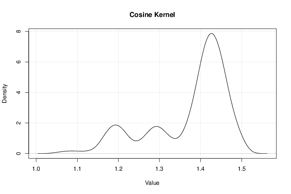
Title produced by software

Kernel Density Estimation

Date of computation

Thu, 29 Sep 2016 15:23:13 +0100

Cite this page as follows

Statistical Computations at FreeStatistics.org, Office for Research Development and Education, URL https://freestatistics.org/blog/index.php?v=date/2016/Sep/29/t1475159010hywrd0uvsklwe0e.htm/, Retrieved Sat, 04 May 2024 22:44:53 +0200

Statistical Computations at FreeStatistics.org, Office for Research Development and Education, URL https://freestatistics.org/blog/index.php?pk=, Retrieved Sat, 04 May 2024 22:44:53 +0200

QR Codes:

Paste this QR Code to cite your computation.

Original text written by user:

IsPrivate?

No (this computation is public)

User-defined keywords

Estimated Impact

Dataseries X:

Download CSV

Histogram

Boxplots

Summary of computational transaction
Raw Input	view raw input (R code)
Raw Output	view raw output of R engine
Computing time	4 seconds
R Server	'Herman Ole Andreas Wold' @ wold.wessa.net

\begin{tabular}{lllllllll}
\hline
Summary of computational transaction \tabularnewline
Raw Input & view raw input (R code)  \tabularnewline
Raw Output & view raw output of R engine  \tabularnewline
Computing time & 4 seconds \tabularnewline
R Server & 'Herman Ole Andreas Wold' @ wold.wessa.net \tabularnewline
\hline
\end{tabular}
%Source: https://freestatistics.org/blog/index.php?pk=&T=0

[TABLE]
[ROW][C]Summary of computational transaction[/C][/ROW]
[ROW][C]Raw Input[/C][C]view raw input (R code) [/C][/ROW]
[ROW][C]Raw Output[/C][C]view raw output of R engine [/C][/ROW]
[ROW][C]Computing time[/C][C]4 seconds[/C][/ROW]
[ROW][C]R Server[/C][C]'Herman Ole Andreas Wold' @ wold.wessa.net[/C][/ROW]
[/TABLE]
Source: https://freestatistics.org/blog/index.php?pk=&T=0

Globally Unique Identifier (entire table): ba.freestatistics.org/blog/index.php?pk=&T=0

As an alternative you can also use a QR Code:

The GUIDs for individual cells are displayed in the table below:

Summary of computational transaction
Raw Input	view raw input (R code)
Raw Output	view raw output of R engine
Computing time	4 seconds
R Server	'Herman Ole Andreas Wold' @ wold.wessa.net

Properties of Density Trace
Bandwidth	0.0200242275489204
#Observations	1461

\begin{tabular}{lllllllll}
\hline
Properties of Density Trace \tabularnewline
Bandwidth & 0.0200242275489204 \tabularnewline
#Observations & 1461 \tabularnewline
\hline
\end{tabular}
%Source: https://freestatistics.org/blog/index.php?pk=&T=1

[TABLE]
[ROW][C]Properties of Density Trace[/C][/ROW]
[ROW][C]Bandwidth[/C][C]0.0200242275489204[/C][/ROW]
[ROW][C]#Observations[/C][C]1461[/C][/ROW]
[/TABLE]
Source: https://freestatistics.org/blog/index.php?pk=&T=1

Globally Unique Identifier (entire table): ba.freestatistics.org/blog/index.php?pk=&T=1

As an alternative you can also use a QR Code:

The GUIDs for individual cells are displayed in the table below:

Properties of Density Trace
Bandwidth	0.0200242275489204
#Observations	1461

Maximum Density Values
Kernel	x-value	max. density
Gaussian	1.4266323200315	8.03898413878181
Epanechnikov	1.42554005904267	7.74788508824208
Rectangular	1.42444779805384	7.61616762208085
Triangular	1.4266323200315	7.91931073062903
Biweight	1.4266323200315	7.8367858929572
Cosine	1.4266323200315	7.86975683434157
Optcosine	1.42554005904267	7.77232799468233

\begin{tabular}{lllllllll}
\hline
Maximum Density Values \tabularnewline
Kernel & x-value & max. density \tabularnewline
Gaussian & 1.4266323200315 & 8.03898413878181 \tabularnewline
Epanechnikov & 1.42554005904267 & 7.74788508824208 \tabularnewline
Rectangular & 1.42444779805384 & 7.61616762208085 \tabularnewline
Triangular & 1.4266323200315 & 7.91931073062903 \tabularnewline
Biweight & 1.4266323200315 & 7.8367858929572 \tabularnewline
Cosine & 1.4266323200315 & 7.86975683434157 \tabularnewline
Optcosine & 1.42554005904267 & 7.77232799468233 \tabularnewline
\hline
\end{tabular}
%Source: https://freestatistics.org/blog/index.php?pk=&T=2

[TABLE]
[ROW][C]Maximum Density Values[/C][/ROW]
[ROW][C]Kernel[/C][C]x-value[/C][C]max. density[/C][/ROW]
[ROW][C]Gaussian[/C][C]1.4266323200315[/C][C]8.03898413878181[/C][/ROW]
[ROW][C]Epanechnikov[/C][C]1.42554005904267[/C][C]7.74788508824208[/C][/ROW]
[ROW][C]Rectangular[/C][C]1.42444779805384[/C][C]7.61616762208085[/C][/ROW]
[ROW][C]Triangular[/C][C]1.4266323200315[/C][C]7.91931073062903[/C][/ROW]
[ROW][C]Biweight[/C][C]1.4266323200315[/C][C]7.8367858929572[/C][/ROW]
[ROW][C]Cosine[/C][C]1.4266323200315[/C][C]7.86975683434157[/C][/ROW]
[ROW][C]Optcosine[/C][C]1.42554005904267[/C][C]7.77232799468233[/C][/ROW]
[/TABLE]
Source: https://freestatistics.org/blog/index.php?pk=&T=2

Globally Unique Identifier (entire table): ba.freestatistics.org/blog/index.php?pk=&T=2

As an alternative you can also use a QR Code:

The GUIDs for individual cells are displayed in the table below:

Maximum Density Values
Kernel	x-value	max. density
Gaussian	1.4266323200315	8.03898413878181
Epanechnikov	1.42554005904267	7.74788508824208
Rectangular	1.42444779805384	7.61616762208085
Triangular	1.4266323200315	7.91931073062903
Biweight	1.4266323200315	7.8367858929572
Cosine	1.4266323200315	7.86975683434157
Optcosine	1.42554005904267	7.77232799468233

Kernel Density Values
x-value	Gaussian	Epanechnikov	Rectangular	Triangular	Biweight	Cosine	Optcosine
Kernel Density Values are not shown

\begin{tabular}{lllllllll}
\hline
Kernel Density Values \tabularnewline
x-value & Gaussian & Epanechnikov & Rectangular & Triangular & Biweight & Cosine & Optcosine \tabularnewline
Kernel Density Values are not shown \tabularnewline
\hline
\end{tabular}
%Source: https://freestatistics.org/blog/index.php?pk=&T=3

[TABLE]
[ROW][C]Kernel Density Values[/C][/ROW]
[ROW][C]x-value[/C][C]Gaussian[/C][C]Epanechnikov[/C][C]Rectangular[/C][C]Triangular[/C][C]Biweight[/C][C]Cosine[/C][C]Optcosine[/C][/ROW]
[ROW][C]Kernel Density Values are not shown[/C][/ROW]
[/TABLE]
Source: https://freestatistics.org/blog/index.php?pk=&T=3

Globally Unique Identifier (entire table): ba.freestatistics.org/blog/index.php?pk=&T=3

As an alternative you can also use a QR Code:

The GUIDs for individual cells are displayed in the table below:

Kernel Density Values
x-value	Gaussian	Epanechnikov	Rectangular	Triangular	Biweight	Cosine	Optcosine
Kernel Density Values are not shown

Figure 1

PNG link

Postscript link

PDF link

Figure 2

PNG link

Postscript link

PDF link

Figure 3

PNG link

Postscript link

PDF link

Figure 4

PNG link

Postscript link

PDF link

Figure 5

PNG link

Postscript link

PDF link

Figure 6

PNG link

Postscript link

PDF link

Figure 7

PNG link

Postscript link

PDF link

Parameters (Session):

par1 = 0 ; par2 = no ; par3 = 512 ;

Parameters (R input):

par1 = 0 ; par2 = no ; par3 = 512 ;

R code (references can be found in the software module):

if (par1 == '0') bw <- 'nrd0'
if (par1 != '0') bw <- as.numeric(par1)
par3 <- as.numeric(par3)
mydensity <- array(NA, dim=c(par3,8))
bitmap(file='density1.png')
mydensity1<-density(x,bw=bw,kernel='gaussian',na.rm=TRUE)
mydensity[,8] = signif(mydensity1$x,3)
mydensity[,1] = signif(mydensity1$y,3)
plot(mydensity1,main='Gaussian Kernel',xlab=xlab,ylab=ylab)
grid()
dev.off()
mydensity1
bitmap(file='density2.png')
mydensity2<-density(x,bw=bw,kernel='epanechnikov',na.rm=TRUE)
mydensity[,2] = signif(mydensity2$y,3)
plot(mydensity2,main='Epanechnikov Kernel',xlab=xlab,ylab=ylab)
grid()
dev.off()
bitmap(file='density3.png')
mydensity3<-density(x,bw=bw,kernel='rectangular',na.rm=TRUE)
mydensity[,3] = signif(mydensity3$y,3)
plot(mydensity3,main='Rectangular Kernel',xlab=xlab,ylab=ylab)
grid()
dev.off()
bitmap(file='density4.png')
mydensity4<-density(x,bw=bw,kernel='triangular',na.rm=TRUE)
mydensity[,4] = signif(mydensity4$y,3)
plot(mydensity4,main='Triangular Kernel',xlab=xlab,ylab=ylab)
grid()
dev.off()
bitmap(file='density5.png')
mydensity5<-density(x,bw=bw,kernel='biweight',na.rm=TRUE)
mydensity[,5] = signif(mydensity5$y,3)
plot(mydensity5,main='Biweight Kernel',xlab=xlab,ylab=ylab)
grid()
dev.off()
bitmap(file='density6.png')
mydensity6<-density(x,bw=bw,kernel='cosine',na.rm=TRUE)
mydensity[,6] = signif(mydensity6$y,3)
plot(mydensity6,main='Cosine Kernel',xlab=xlab,ylab=ylab)
grid()
dev.off()
bitmap(file='density7.png')
mydensity7<-density(x,bw=bw,kernel='optcosine',na.rm=TRUE)
mydensity[,7] = signif(mydensity7$y,3)
plot(mydensity7,main='Optcosine Kernel',xlab=xlab,ylab=ylab)
grid()
dev.off()
load(file='createtable')
ab<-table.start()
ab<-table.row.start(ab)
ab<-table.element(ab,'Properties of Density Trace',2,TRUE)
ab<-table.row.end(ab)
ab<-table.row.start(ab)
ab<-table.element(ab,'Bandwidth',header=TRUE)
ab<-table.element(ab,mydensity1$bw)
ab<-table.row.end(ab)
ab<-table.row.start(ab)
ab<-table.element(ab,'#Observations',header=TRUE)
ab<-table.element(ab,mydensity1$n)
ab<-table.row.end(ab)
ab<-table.end(ab)
a <- ab
table.save(ab,file='mytable123.tab')
b<-table.start()
b<-table.row.start(b)
b<-table.element(b,'Maximum Density Values',3,TRUE)
b<-table.row.end(b)
b<-table.row.start(b)
b<-table.element(b,'Kernel',1,TRUE)
b<-table.element(b,'x-value',1,TRUE)
b<-table.element(b,'max. density',1,TRUE)
b<-table.row.end(b)
b<-table.row.start(b)
b<-table.element(b,'Gaussian',1,TRUE)
b<-table.element(b,mydensity1$x[mydensity1$y==max(mydensity1$y)],1)
b<-table.element(b,mydensity1$y[mydensity1$y==max(mydensity1$y)],1)
b<-table.row.end(b)
b<-table.row.start(b)
b<-table.element(b,'Epanechnikov',1,TRUE)
b<-table.element(b,mydensity2$x[mydensity2$y==max(mydensity2$y)],1)
b<-table.element(b,mydensity2$y[mydensity2$y==max(mydensity2$y)],1)
b<-table.row.end(b)
b<-table.row.start(b)
b<-table.element(b,'Rectangular',1,TRUE)
b<-table.element(b,mydensity3$x[mydensity3$y==max(mydensity3$y)],1)
b<-table.element(b,mydensity3$y[mydensity3$y==max(mydensity3$y)],1)
b<-table.row.end(b)
b<-table.row.start(b)
b<-table.element(b,'Triangular',1,TRUE)
b<-table.element(b,mydensity4$x[mydensity4$y==max(mydensity4$y)],1)
b<-table.element(b,mydensity4$y[mydensity4$y==max(mydensity4$y)],1)
b<-table.row.end(b)
b<-table.row.start(b)
b<-table.element(b,'Biweight',1,TRUE)
b<-table.element(b,mydensity5$x[mydensity5$y==max(mydensity5$y)],1)
b<-table.element(b,mydensity5$y[mydensity5$y==max(mydensity5$y)],1)
b<-table.row.end(b)
b<-table.row.start(b)
b<-table.element(b,'Cosine',1,TRUE)
b<-table.element(b,mydensity6$x[mydensity6$y==max(mydensity6$y)],1)
b<-table.element(b,mydensity6$y[mydensity6$y==max(mydensity6$y)],1)
b<-table.row.end(b)
b<-table.row.start(b)
b<-table.element(b,'Optcosine',1,TRUE)
b<-table.element(b,mydensity7$x[mydensity7$y==max(mydensity7$y)],1)
b<-table.element(b,mydensity7$y[mydensity7$y==max(mydensity7$y)],1)
b<-table.row.end(b)
b<-table.end(b)
a <- b[1]
table.save(b,file='mytable2a.tab')
a<-table.start()
a<-table.row.start(a)
a<-table.element(a,'Kernel Density Values',8,TRUE)
a<-table.row.end(a)
a<-table.row.start(a)
a<-table.element(a,'x-value',1,TRUE)
a<-table.element(a,'Gaussian',1,TRUE)
a<-table.element(a,'Epanechnikov',1,TRUE)
a<-table.element(a,'Rectangular',1,TRUE)
a<-table.element(a,'Triangular',1,TRUE)
a<-table.element(a,'Biweight',1,TRUE)
a<-table.element(a,'Cosine',1,TRUE)
a<-table.element(a,'Optcosine',1,TRUE)
a<-table.row.end(a)
if (par2=='yes') {
for(i in 1:par3) {
a<-table.row.start(a)
a<-table.element(a,mydensity[i,8],1,TRUE)
for(j in 1:7) {
a<-table.element(a,mydensity[i,j],1)
}
a<-table.row.end(a)
}
} else {
a<-table.row.start(a)
a<-table.element(a,'Kernel Density Values are not shown',8)
a<-table.row.end(a)
}
a<-table.end(a)
table.save(a,file='mytable1.tab')

Free Statistics

Description of Statistical Computation

Tree of Dependent Computations

Dataset

Tables (Output of Computation)

Figures (Output of Computation)

Input Parameters & R Code