Repository of Reproducible Computations

Free Statistics

of Irreproducible Research!

Author's title

Author

*The author of this computation has been verified*

R Software Module

rwasp_autocorrelation.wasp

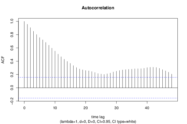
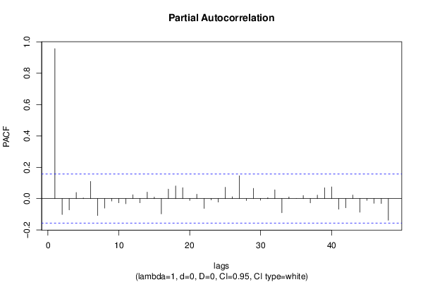
Title produced by software

(Partial) Autocorrelation Function

Date of computation

Sun, 08 Jan 2017 16:38:50 +0000

Cite this page as follows

Statistical Computations at FreeStatistics.org, Office for Research Development and Education, URL https://freestatistics.org/blog/index.php?v=date/2017/Jan/08/t1483893588l8ebd5b3l09kb7u.htm/, Retrieved Tue, 14 May 2024 05:30:52 +0200

Statistical Computations at FreeStatistics.org, Office for Research Development and Education, URL https://freestatistics.org/blog/index.php?pk=, Retrieved Tue, 14 May 2024 05:30:52 +0200

QR Codes:

Paste this QR Code to cite your computation.

Original text written by user:

IsPrivate?

No (this computation is public)

User-defined keywords

Estimated Impact

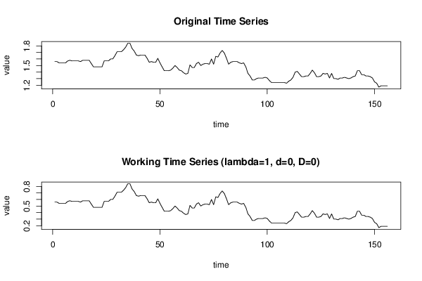
Dataseries X:

Download CSV

Histogram

Boxplots

1,56
1,56
1,54
1,54
1,54
1,54
1,57
1,58
1,57
1,57
1,57
1,57
1,56
1,58
1,58
1,58
1,58
1,53
1,48
1,48
1,48
1,48
1,48
1,57
1,57
1,57
1,60
1,60
1,65
1,71
1,71
1,71
1,74
1,78
1,84
1,84
1,76
1,72
1,66
1,65
1,66
1,66
1,66
1,61
1,55
1,56
1,55
1,55
1,61
1,54
1,48
1,42
1,42
1,42
1,43
1,46
1,50
1,47
1,43
1,42
1,39
1,37
1,38
1,51
1,47
1,47
1,53
1,55
1,50
1,52
1,53
1,53
1,52
1,60
1,52
1,64
1,63
1,69
1,73
1,69
1,61
1,52
1,55
1,56
1,56
1,56
1,54
1,53
1,54
1,48
1,38
1,34
1,28
1,28
1,30
1,31
1,31
1,31
1,32
1,31
1,27
1,24
1,24
1,24
1,24
1,24
1,24
1,24
1,23
1,26
1,28
1,32
1,40
1,41
1,37
1,33
1,33
1,34
1,34
1,38
1,43
1,39
1,33
1,33
1,34
1,38
1,37
1,38
1,31
1,38
1,30
1,30
1,29
1,31
1,31
1,32
1,31
1,30
1,31
1,33
1,34
1,42
1,42
1,36
1,36
1,34
1,34
1,33
1,31
1,25
1,23
1,17
1,19
1,19
1,19
1,19

Summary of computational transaction
Raw Input	view raw input (R code)
Raw Output	view raw output of R engine
Computing time	1 seconds
R Server	'Herman Ole Andreas Wold' @ wold.wessa.net

\begin{tabular}{lllllllll}
\hline
Summary of computational transaction \tabularnewline
Raw Input & view raw input (R code)  \tabularnewline
Raw Output & view raw output of R engine  \tabularnewline
Computing time & 1 seconds \tabularnewline
R Server & 'Herman Ole Andreas Wold' @ wold.wessa.net \tabularnewline
\hline
\end{tabular}
%Source: https://freestatistics.org/blog/index.php?pk=&T=0

[TABLE]
[ROW][C]Summary of computational transaction[/C][/ROW]
[ROW][C]Raw Input[/C][C]view raw input (R code) [/C][/ROW]
[ROW][C]Raw Output[/C][C]view raw output of R engine [/C][/ROW]
[ROW][C]Computing time[/C][C]1 seconds[/C][/ROW]
[ROW][C]R Server[/C][C]'Herman Ole Andreas Wold' @ wold.wessa.net[/C][/ROW]
[/TABLE]
Source: https://freestatistics.org/blog/index.php?pk=&T=0

Globally Unique Identifier (entire table): ba.freestatistics.org/blog/index.php?pk=&T=0

As an alternative you can also use a QR Code:

The GUIDs for individual cells are displayed in the table below:

Summary of computational transaction
Raw Input	view raw input (R code)
Raw Output	view raw output of R engine
Computing time	1 seconds
R Server	'Herman Ole Andreas Wold' @ wold.wessa.net

Autocorrelation Function
Time lag k	ACF(k)	T-STAT	P-value
1	0.95651	11.9468	0
2	0.906287	11.3195	0
3	0.851743	10.6383	0
4	0.802411	10.0221	0
5	0.756338	9.4467	0
6	0.722607	9.0254	0
7	0.683307	8.5345	0
8	0.6409	8.0048	0
9	0.596906	7.4554	0
10	0.552621	6.9022	0
11	0.506955	6.3319	0
12	0.467554	5.8397	0
13	0.429374	5.3629	0
14	0.397206	4.9611	1e-06
15	0.368165	4.5984	4e-06
16	0.334098	4.1729	2.5e-05
17	0.304295	3.8006	0.000103
18	0.283235	3.5376	0.000266
19	0.270597	3.3798	0.000458
20	0.260064	3.2482	0.000711
21	0.255297	3.1887	0.000864
22	0.244256	3.0508	0.001342
23	0.230539	2.8794	0.002272
24	0.214701	2.6816	0.004058
25	0.206714	2.5819	0.005374
26	0.200755	2.5074	0.006592
27	0.210897	2.6341	0.004643
28	0.221412	2.7654	0.003185
29	0.237903	2.9714	0.001717
30	0.249727	3.1191	0.001081
31	0.259964	3.2469	0.000714
32	0.268914	3.3587	0.000492
33	0.273421	3.415	0.000407
34	0.277019	3.46	0.000348
35	0.280844	3.5077	0.000295
36	0.285674	3.5681	0.000239
37	0.287047	3.5852	0.000225
38	0.288239	3.6001	0.000213
39	0.293656	3.6678	0.000168
40	0.303826	3.7948	0.000106
41	0.308604	3.8545	8.5e-05
42	0.309148	3.8613	8.2e-05
43	0.30571	3.8183	9.7e-05
44	0.292692	3.6557	0.000175
45	0.273689	3.4184	0.000402
46	0.255051	3.1856	0.000872
47	0.234497	2.9289	0.001956
48	0.205518	2.5669	0.005601

\begin{tabular}{lllllllll}
\hline
Autocorrelation Function \tabularnewline
Time lag k & ACF(k) & T-STAT & P-value \tabularnewline
1 & 0.95651 & 11.9468 & 0 \tabularnewline
2 & 0.906287 & 11.3195 & 0 \tabularnewline
3 & 0.851743 & 10.6383 & 0 \tabularnewline
4 & 0.802411 & 10.0221 & 0 \tabularnewline
5 & 0.756338 & 9.4467 & 0 \tabularnewline
6 & 0.722607 & 9.0254 & 0 \tabularnewline
7 & 0.683307 & 8.5345 & 0 \tabularnewline
8 & 0.6409 & 8.0048 & 0 \tabularnewline
9 & 0.596906 & 7.4554 & 0 \tabularnewline
10 & 0.552621 & 6.9022 & 0 \tabularnewline
11 & 0.506955 & 6.3319 & 0 \tabularnewline
12 & 0.467554 & 5.8397 & 0 \tabularnewline
13 & 0.429374 & 5.3629 & 0 \tabularnewline
14 & 0.397206 & 4.9611 & 1e-06 \tabularnewline
15 & 0.368165 & 4.5984 & 4e-06 \tabularnewline
16 & 0.334098 & 4.1729 & 2.5e-05 \tabularnewline
17 & 0.304295 & 3.8006 & 0.000103 \tabularnewline
18 & 0.283235 & 3.5376 & 0.000266 \tabularnewline
19 & 0.270597 & 3.3798 & 0.000458 \tabularnewline
20 & 0.260064 & 3.2482 & 0.000711 \tabularnewline
21 & 0.255297 & 3.1887 & 0.000864 \tabularnewline
22 & 0.244256 & 3.0508 & 0.001342 \tabularnewline
23 & 0.230539 & 2.8794 & 0.002272 \tabularnewline
24 & 0.214701 & 2.6816 & 0.004058 \tabularnewline
25 & 0.206714 & 2.5819 & 0.005374 \tabularnewline
26 & 0.200755 & 2.5074 & 0.006592 \tabularnewline
27 & 0.210897 & 2.6341 & 0.004643 \tabularnewline
28 & 0.221412 & 2.7654 & 0.003185 \tabularnewline
29 & 0.237903 & 2.9714 & 0.001717 \tabularnewline
30 & 0.249727 & 3.1191 & 0.001081 \tabularnewline
31 & 0.259964 & 3.2469 & 0.000714 \tabularnewline
32 & 0.268914 & 3.3587 & 0.000492 \tabularnewline
33 & 0.273421 & 3.415 & 0.000407 \tabularnewline
34 & 0.277019 & 3.46 & 0.000348 \tabularnewline
35 & 0.280844 & 3.5077 & 0.000295 \tabularnewline
36 & 0.285674 & 3.5681 & 0.000239 \tabularnewline
37 & 0.287047 & 3.5852 & 0.000225 \tabularnewline
38 & 0.288239 & 3.6001 & 0.000213 \tabularnewline
39 & 0.293656 & 3.6678 & 0.000168 \tabularnewline
40 & 0.303826 & 3.7948 & 0.000106 \tabularnewline
41 & 0.308604 & 3.8545 & 8.5e-05 \tabularnewline
42 & 0.309148 & 3.8613 & 8.2e-05 \tabularnewline
43 & 0.30571 & 3.8183 & 9.7e-05 \tabularnewline
44 & 0.292692 & 3.6557 & 0.000175 \tabularnewline
45 & 0.273689 & 3.4184 & 0.000402 \tabularnewline
46 & 0.255051 & 3.1856 & 0.000872 \tabularnewline
47 & 0.234497 & 2.9289 & 0.001956 \tabularnewline
48 & 0.205518 & 2.5669 & 0.005601 \tabularnewline
\hline
\end{tabular}
%Source: https://freestatistics.org/blog/index.php?pk=&T=1

[TABLE]
[ROW][C]Autocorrelation Function[/C][/ROW]
[ROW][C]Time lag k[/C][C]ACF(k)[/C][C]T-STAT[/C][C]P-value[/C][/ROW]
[ROW][C]1[/C][C]0.95651[/C][C]11.9468[/C][C]0[/C][/ROW]
[ROW][C]2[/C][C]0.906287[/C][C]11.3195[/C][C]0[/C][/ROW]
[ROW][C]3[/C][C]0.851743[/C][C]10.6383[/C][C]0[/C][/ROW]
[ROW][C]4[/C][C]0.802411[/C][C]10.0221[/C][C]0[/C][/ROW]
[ROW][C]5[/C][C]0.756338[/C][C]9.4467[/C][C]0[/C][/ROW]
[ROW][C]6[/C][C]0.722607[/C][C]9.0254[/C][C]0[/C][/ROW]
[ROW][C]7[/C][C]0.683307[/C][C]8.5345[/C][C]0[/C][/ROW]
[ROW][C]8[/C][C]0.6409[/C][C]8.0048[/C][C]0[/C][/ROW]
[ROW][C]9[/C][C]0.596906[/C][C]7.4554[/C][C]0[/C][/ROW]
[ROW][C]10[/C][C]0.552621[/C][C]6.9022[/C][C]0[/C][/ROW]
[ROW][C]11[/C][C]0.506955[/C][C]6.3319[/C][C]0[/C][/ROW]
[ROW][C]12[/C][C]0.467554[/C][C]5.8397[/C][C]0[/C][/ROW]
[ROW][C]13[/C][C]0.429374[/C][C]5.3629[/C][C]0[/C][/ROW]
[ROW][C]14[/C][C]0.397206[/C][C]4.9611[/C][C]1e-06[/C][/ROW]
[ROW][C]15[/C][C]0.368165[/C][C]4.5984[/C][C]4e-06[/C][/ROW]
[ROW][C]16[/C][C]0.334098[/C][C]4.1729[/C][C]2.5e-05[/C][/ROW]
[ROW][C]17[/C][C]0.304295[/C][C]3.8006[/C][C]0.000103[/C][/ROW]
[ROW][C]18[/C][C]0.283235[/C][C]3.5376[/C][C]0.000266[/C][/ROW]
[ROW][C]19[/C][C]0.270597[/C][C]3.3798[/C][C]0.000458[/C][/ROW]
[ROW][C]20[/C][C]0.260064[/C][C]3.2482[/C][C]0.000711[/C][/ROW]
[ROW][C]21[/C][C]0.255297[/C][C]3.1887[/C][C]0.000864[/C][/ROW]
[ROW][C]22[/C][C]0.244256[/C][C]3.0508[/C][C]0.001342[/C][/ROW]
[ROW][C]23[/C][C]0.230539[/C][C]2.8794[/C][C]0.002272[/C][/ROW]
[ROW][C]24[/C][C]0.214701[/C][C]2.6816[/C][C]0.004058[/C][/ROW]
[ROW][C]25[/C][C]0.206714[/C][C]2.5819[/C][C]0.005374[/C][/ROW]
[ROW][C]26[/C][C]0.200755[/C][C]2.5074[/C][C]0.006592[/C][/ROW]
[ROW][C]27[/C][C]0.210897[/C][C]2.6341[/C][C]0.004643[/C][/ROW]
[ROW][C]28[/C][C]0.221412[/C][C]2.7654[/C][C]0.003185[/C][/ROW]
[ROW][C]29[/C][C]0.237903[/C][C]2.9714[/C][C]0.001717[/C][/ROW]
[ROW][C]30[/C][C]0.249727[/C][C]3.1191[/C][C]0.001081[/C][/ROW]
[ROW][C]31[/C][C]0.259964[/C][C]3.2469[/C][C]0.000714[/C][/ROW]
[ROW][C]32[/C][C]0.268914[/C][C]3.3587[/C][C]0.000492[/C][/ROW]
[ROW][C]33[/C][C]0.273421[/C][C]3.415[/C][C]0.000407[/C][/ROW]
[ROW][C]34[/C][C]0.277019[/C][C]3.46[/C][C]0.000348[/C][/ROW]
[ROW][C]35[/C][C]0.280844[/C][C]3.5077[/C][C]0.000295[/C][/ROW]
[ROW][C]36[/C][C]0.285674[/C][C]3.5681[/C][C]0.000239[/C][/ROW]
[ROW][C]37[/C][C]0.287047[/C][C]3.5852[/C][C]0.000225[/C][/ROW]
[ROW][C]38[/C][C]0.288239[/C][C]3.6001[/C][C]0.000213[/C][/ROW]
[ROW][C]39[/C][C]0.293656[/C][C]3.6678[/C][C]0.000168[/C][/ROW]
[ROW][C]40[/C][C]0.303826[/C][C]3.7948[/C][C]0.000106[/C][/ROW]
[ROW][C]41[/C][C]0.308604[/C][C]3.8545[/C][C]8.5e-05[/C][/ROW]
[ROW][C]42[/C][C]0.309148[/C][C]3.8613[/C][C]8.2e-05[/C][/ROW]
[ROW][C]43[/C][C]0.30571[/C][C]3.8183[/C][C]9.7e-05[/C][/ROW]
[ROW][C]44[/C][C]0.292692[/C][C]3.6557[/C][C]0.000175[/C][/ROW]
[ROW][C]45[/C][C]0.273689[/C][C]3.4184[/C][C]0.000402[/C][/ROW]
[ROW][C]46[/C][C]0.255051[/C][C]3.1856[/C][C]0.000872[/C][/ROW]
[ROW][C]47[/C][C]0.234497[/C][C]2.9289[/C][C]0.001956[/C][/ROW]
[ROW][C]48[/C][C]0.205518[/C][C]2.5669[/C][C]0.005601[/C][/ROW]
[/TABLE]
Source: https://freestatistics.org/blog/index.php?pk=&T=1

Globally Unique Identifier (entire table): ba.freestatistics.org/blog/index.php?pk=&T=1

As an alternative you can also use a QR Code:

The GUIDs for individual cells are displayed in the table below:

Autocorrelation Function
Time lag k	ACF(k)	T-STAT	P-value
1	0.95651	11.9468	0
2	0.906287	11.3195	0
3	0.851743	10.6383	0
4	0.802411	10.0221	0
5	0.756338	9.4467	0
6	0.722607	9.0254	0
7	0.683307	8.5345	0
8	0.6409	8.0048	0
9	0.596906	7.4554	0
10	0.552621	6.9022	0
11	0.506955	6.3319	0
12	0.467554	5.8397	0
13	0.429374	5.3629	0
14	0.397206	4.9611	1e-06
15	0.368165	4.5984	4e-06
16	0.334098	4.1729	2.5e-05
17	0.304295	3.8006	0.000103
18	0.283235	3.5376	0.000266
19	0.270597	3.3798	0.000458
20	0.260064	3.2482	0.000711
21	0.255297	3.1887	0.000864
22	0.244256	3.0508	0.001342
23	0.230539	2.8794	0.002272
24	0.214701	2.6816	0.004058
25	0.206714	2.5819	0.005374
26	0.200755	2.5074	0.006592
27	0.210897	2.6341	0.004643
28	0.221412	2.7654	0.003185
29	0.237903	2.9714	0.001717
30	0.249727	3.1191	0.001081
31	0.259964	3.2469	0.000714
32	0.268914	3.3587	0.000492
33	0.273421	3.415	0.000407
34	0.277019	3.46	0.000348
35	0.280844	3.5077	0.000295
36	0.285674	3.5681	0.000239
37	0.287047	3.5852	0.000225
38	0.288239	3.6001	0.000213
39	0.293656	3.6678	0.000168
40	0.303826	3.7948	0.000106
41	0.308604	3.8545	8.5e-05
42	0.309148	3.8613	8.2e-05
43	0.30571	3.8183	9.7e-05
44	0.292692	3.6557	0.000175
45	0.273689	3.4184	0.000402
46	0.255051	3.1856	0.000872
47	0.234497	2.9289	0.001956
48	0.205518	2.5669	0.005601

Partial Autocorrelation Function
Time lag k	PACF(k)	T-STAT	P-value
1	0.95651	11.9468	0
2	-0.101368	-1.2661	0.103685
3	-0.071765	-0.8963	0.185726
4	0.039592	0.4945	0.310825
5	0.004365	0.0545	0.478295
6	0.109715	1.3703	0.086276
7	-0.108069	-1.3498	0.08952
8	-0.060283	-0.7529	0.226313
9	-0.015249	-0.1905	0.424598
10	-0.026554	-0.3317	0.370295
11	-0.03238	-0.4044	0.343228
12	0.024918	0.3112	0.378022
13	-0.026428	-0.3301	0.370888
14	0.041937	0.5238	0.300584
15	0.00969	0.121	0.451912
16	-0.097287	-1.2151	0.113079
17	0.06045	0.755	0.225686
18	0.08107	1.0126	0.156419
19	0.069763	0.8713	0.192455
20	-0.011723	-0.1464	0.44189
21	0.028435	0.3552	0.361478
22	-0.062317	-0.7783	0.218774
23	-0.008547	-0.1067	0.457563
24	-0.022038	-0.2753	0.39174
25	0.072425	0.9046	0.18354
26	0.011673	0.1458	0.442133
27	0.145592	1.8184	0.035458
28	-0.01217	-0.152	0.439692
29	0.065602	0.8194	0.206914
30	-0.010151	-0.1268	0.449639
31	0.006186	0.0773	0.469255
32	0.056107	0.7008	0.242244
33	-0.089997	-1.1241	0.131357
34	0.010826	0.1352	0.446307
35	0.00055	0.0069	0.497264
36	0.019687	0.2459	0.403046
37	-0.026805	-0.3348	0.369115
38	0.02224	0.2778	0.390776
39	0.069263	0.8651	0.194159
40	0.074882	0.9353	0.175546
41	-0.067145	-0.8386	0.201478
42	-0.058243	-0.7275	0.234018
43	0.023158	0.2892	0.386391
44	-0.086552	-1.081	0.140674
45	-0.011542	-0.1442	0.442782
46	-0.029908	-0.3735	0.354625
47	-0.03104	-0.3877	0.349385
48	-0.137775	-1.7208	0.043634

\begin{tabular}{lllllllll}
\hline
Partial Autocorrelation Function \tabularnewline
Time lag k & PACF(k) & T-STAT & P-value \tabularnewline
1 & 0.95651 & 11.9468 & 0 \tabularnewline
2 & -0.101368 & -1.2661 & 0.103685 \tabularnewline
3 & -0.071765 & -0.8963 & 0.185726 \tabularnewline
4 & 0.039592 & 0.4945 & 0.310825 \tabularnewline
5 & 0.004365 & 0.0545 & 0.478295 \tabularnewline
6 & 0.109715 & 1.3703 & 0.086276 \tabularnewline
7 & -0.108069 & -1.3498 & 0.08952 \tabularnewline
8 & -0.060283 & -0.7529 & 0.226313 \tabularnewline
9 & -0.015249 & -0.1905 & 0.424598 \tabularnewline
10 & -0.026554 & -0.3317 & 0.370295 \tabularnewline
11 & -0.03238 & -0.4044 & 0.343228 \tabularnewline
12 & 0.024918 & 0.3112 & 0.378022 \tabularnewline
13 & -0.026428 & -0.3301 & 0.370888 \tabularnewline
14 & 0.041937 & 0.5238 & 0.300584 \tabularnewline
15 & 0.00969 & 0.121 & 0.451912 \tabularnewline
16 & -0.097287 & -1.2151 & 0.113079 \tabularnewline
17 & 0.06045 & 0.755 & 0.225686 \tabularnewline
18 & 0.08107 & 1.0126 & 0.156419 \tabularnewline
19 & 0.069763 & 0.8713 & 0.192455 \tabularnewline
20 & -0.011723 & -0.1464 & 0.44189 \tabularnewline
21 & 0.028435 & 0.3552 & 0.361478 \tabularnewline
22 & -0.062317 & -0.7783 & 0.218774 \tabularnewline
23 & -0.008547 & -0.1067 & 0.457563 \tabularnewline
24 & -0.022038 & -0.2753 & 0.39174 \tabularnewline
25 & 0.072425 & 0.9046 & 0.18354 \tabularnewline
26 & 0.011673 & 0.1458 & 0.442133 \tabularnewline
27 & 0.145592 & 1.8184 & 0.035458 \tabularnewline
28 & -0.01217 & -0.152 & 0.439692 \tabularnewline
29 & 0.065602 & 0.8194 & 0.206914 \tabularnewline
30 & -0.010151 & -0.1268 & 0.449639 \tabularnewline
31 & 0.006186 & 0.0773 & 0.469255 \tabularnewline
32 & 0.056107 & 0.7008 & 0.242244 \tabularnewline
33 & -0.089997 & -1.1241 & 0.131357 \tabularnewline
34 & 0.010826 & 0.1352 & 0.446307 \tabularnewline
35 & 0.00055 & 0.0069 & 0.497264 \tabularnewline
36 & 0.019687 & 0.2459 & 0.403046 \tabularnewline
37 & -0.026805 & -0.3348 & 0.369115 \tabularnewline
38 & 0.02224 & 0.2778 & 0.390776 \tabularnewline
39 & 0.069263 & 0.8651 & 0.194159 \tabularnewline
40 & 0.074882 & 0.9353 & 0.175546 \tabularnewline
41 & -0.067145 & -0.8386 & 0.201478 \tabularnewline
42 & -0.058243 & -0.7275 & 0.234018 \tabularnewline
43 & 0.023158 & 0.2892 & 0.386391 \tabularnewline
44 & -0.086552 & -1.081 & 0.140674 \tabularnewline
45 & -0.011542 & -0.1442 & 0.442782 \tabularnewline
46 & -0.029908 & -0.3735 & 0.354625 \tabularnewline
47 & -0.03104 & -0.3877 & 0.349385 \tabularnewline
48 & -0.137775 & -1.7208 & 0.043634 \tabularnewline
\hline
\end{tabular}
%Source: https://freestatistics.org/blog/index.php?pk=&T=2

[TABLE]
[ROW][C]Partial Autocorrelation Function[/C][/ROW]
[ROW][C]Time lag k[/C][C]PACF(k)[/C][C]T-STAT[/C][C]P-value[/C][/ROW]
[ROW][C]1[/C][C]0.95651[/C][C]11.9468[/C][C]0[/C][/ROW]
[ROW][C]2[/C][C]-0.101368[/C][C]-1.2661[/C][C]0.103685[/C][/ROW]
[ROW][C]3[/C][C]-0.071765[/C][C]-0.8963[/C][C]0.185726[/C][/ROW]
[ROW][C]4[/C][C]0.039592[/C][C]0.4945[/C][C]0.310825[/C][/ROW]
[ROW][C]5[/C][C]0.004365[/C][C]0.0545[/C][C]0.478295[/C][/ROW]
[ROW][C]6[/C][C]0.109715[/C][C]1.3703[/C][C]0.086276[/C][/ROW]
[ROW][C]7[/C][C]-0.108069[/C][C]-1.3498[/C][C]0.08952[/C][/ROW]
[ROW][C]8[/C][C]-0.060283[/C][C]-0.7529[/C][C]0.226313[/C][/ROW]
[ROW][C]9[/C][C]-0.015249[/C][C]-0.1905[/C][C]0.424598[/C][/ROW]
[ROW][C]10[/C][C]-0.026554[/C][C]-0.3317[/C][C]0.370295[/C][/ROW]
[ROW][C]11[/C][C]-0.03238[/C][C]-0.4044[/C][C]0.343228[/C][/ROW]
[ROW][C]12[/C][C]0.024918[/C][C]0.3112[/C][C]0.378022[/C][/ROW]
[ROW][C]13[/C][C]-0.026428[/C][C]-0.3301[/C][C]0.370888[/C][/ROW]
[ROW][C]14[/C][C]0.041937[/C][C]0.5238[/C][C]0.300584[/C][/ROW]
[ROW][C]15[/C][C]0.00969[/C][C]0.121[/C][C]0.451912[/C][/ROW]
[ROW][C]16[/C][C]-0.097287[/C][C]-1.2151[/C][C]0.113079[/C][/ROW]
[ROW][C]17[/C][C]0.06045[/C][C]0.755[/C][C]0.225686[/C][/ROW]
[ROW][C]18[/C][C]0.08107[/C][C]1.0126[/C][C]0.156419[/C][/ROW]
[ROW][C]19[/C][C]0.069763[/C][C]0.8713[/C][C]0.192455[/C][/ROW]
[ROW][C]20[/C][C]-0.011723[/C][C]-0.1464[/C][C]0.44189[/C][/ROW]
[ROW][C]21[/C][C]0.028435[/C][C]0.3552[/C][C]0.361478[/C][/ROW]
[ROW][C]22[/C][C]-0.062317[/C][C]-0.7783[/C][C]0.218774[/C][/ROW]
[ROW][C]23[/C][C]-0.008547[/C][C]-0.1067[/C][C]0.457563[/C][/ROW]
[ROW][C]24[/C][C]-0.022038[/C][C]-0.2753[/C][C]0.39174[/C][/ROW]
[ROW][C]25[/C][C]0.072425[/C][C]0.9046[/C][C]0.18354[/C][/ROW]
[ROW][C]26[/C][C]0.011673[/C][C]0.1458[/C][C]0.442133[/C][/ROW]
[ROW][C]27[/C][C]0.145592[/C][C]1.8184[/C][C]0.035458[/C][/ROW]
[ROW][C]28[/C][C]-0.01217[/C][C]-0.152[/C][C]0.439692[/C][/ROW]
[ROW][C]29[/C][C]0.065602[/C][C]0.8194[/C][C]0.206914[/C][/ROW]
[ROW][C]30[/C][C]-0.010151[/C][C]-0.1268[/C][C]0.449639[/C][/ROW]
[ROW][C]31[/C][C]0.006186[/C][C]0.0773[/C][C]0.469255[/C][/ROW]
[ROW][C]32[/C][C]0.056107[/C][C]0.7008[/C][C]0.242244[/C][/ROW]
[ROW][C]33[/C][C]-0.089997[/C][C]-1.1241[/C][C]0.131357[/C][/ROW]
[ROW][C]34[/C][C]0.010826[/C][C]0.1352[/C][C]0.446307[/C][/ROW]
[ROW][C]35[/C][C]0.00055[/C][C]0.0069[/C][C]0.497264[/C][/ROW]
[ROW][C]36[/C][C]0.019687[/C][C]0.2459[/C][C]0.403046[/C][/ROW]
[ROW][C]37[/C][C]-0.026805[/C][C]-0.3348[/C][C]0.369115[/C][/ROW]
[ROW][C]38[/C][C]0.02224[/C][C]0.2778[/C][C]0.390776[/C][/ROW]
[ROW][C]39[/C][C]0.069263[/C][C]0.8651[/C][C]0.194159[/C][/ROW]
[ROW][C]40[/C][C]0.074882[/C][C]0.9353[/C][C]0.175546[/C][/ROW]
[ROW][C]41[/C][C]-0.067145[/C][C]-0.8386[/C][C]0.201478[/C][/ROW]
[ROW][C]42[/C][C]-0.058243[/C][C]-0.7275[/C][C]0.234018[/C][/ROW]
[ROW][C]43[/C][C]0.023158[/C][C]0.2892[/C][C]0.386391[/C][/ROW]
[ROW][C]44[/C][C]-0.086552[/C][C]-1.081[/C][C]0.140674[/C][/ROW]
[ROW][C]45[/C][C]-0.011542[/C][C]-0.1442[/C][C]0.442782[/C][/ROW]
[ROW][C]46[/C][C]-0.029908[/C][C]-0.3735[/C][C]0.354625[/C][/ROW]
[ROW][C]47[/C][C]-0.03104[/C][C]-0.3877[/C][C]0.349385[/C][/ROW]
[ROW][C]48[/C][C]-0.137775[/C][C]-1.7208[/C][C]0.043634[/C][/ROW]
[/TABLE]
Source: https://freestatistics.org/blog/index.php?pk=&T=2

Globally Unique Identifier (entire table): ba.freestatistics.org/blog/index.php?pk=&T=2

As an alternative you can also use a QR Code:

The GUIDs for individual cells are displayed in the table below:

Partial Autocorrelation Function
Time lag k	PACF(k)	T-STAT	P-value
1	0.95651	11.9468	0
2	-0.101368	-1.2661	0.103685
3	-0.071765	-0.8963	0.185726
4	0.039592	0.4945	0.310825
5	0.004365	0.0545	0.478295
6	0.109715	1.3703	0.086276
7	-0.108069	-1.3498	0.08952
8	-0.060283	-0.7529	0.226313
9	-0.015249	-0.1905	0.424598
10	-0.026554	-0.3317	0.370295
11	-0.03238	-0.4044	0.343228
12	0.024918	0.3112	0.378022
13	-0.026428	-0.3301	0.370888
14	0.041937	0.5238	0.300584
15	0.00969	0.121	0.451912
16	-0.097287	-1.2151	0.113079
17	0.06045	0.755	0.225686
18	0.08107	1.0126	0.156419
19	0.069763	0.8713	0.192455
20	-0.011723	-0.1464	0.44189
21	0.028435	0.3552	0.361478
22	-0.062317	-0.7783	0.218774
23	-0.008547	-0.1067	0.457563
24	-0.022038	-0.2753	0.39174
25	0.072425	0.9046	0.18354
26	0.011673	0.1458	0.442133
27	0.145592	1.8184	0.035458
28	-0.01217	-0.152	0.439692
29	0.065602	0.8194	0.206914
30	-0.010151	-0.1268	0.449639
31	0.006186	0.0773	0.469255
32	0.056107	0.7008	0.242244
33	-0.089997	-1.1241	0.131357
34	0.010826	0.1352	0.446307
35	0.00055	0.0069	0.497264
36	0.019687	0.2459	0.403046
37	-0.026805	-0.3348	0.369115
38	0.02224	0.2778	0.390776
39	0.069263	0.8651	0.194159
40	0.074882	0.9353	0.175546
41	-0.067145	-0.8386	0.201478
42	-0.058243	-0.7275	0.234018
43	0.023158	0.2892	0.386391
44	-0.086552	-1.081	0.140674
45	-0.011542	-0.1442	0.442782
46	-0.029908	-0.3735	0.354625
47	-0.03104	-0.3877	0.349385
48	-0.137775	-1.7208	0.043634

Figure 1

PNG link

Postscript link

PDF link

Figure 2

PNG link

Postscript link

PDF link

Figure 3

PNG link

Postscript link

PDF link

Parameters (Session):

par1 = 48 ; par2 = 1 ; par3 = 0 ; par4 = 0 ; par5 = 12 ; par6 = White Noise ; par7 = 0.95 ;

Parameters (R input):

par1 = 48 ; par2 = 1 ; par3 = 0 ; par4 = 0 ; par5 = 12 ; par6 = White Noise ; par7 = 0.95 ; par8 = ;

R code (references can be found in the software module):

if (par1 == 'Default') {
par1 = 10*log10(length(x))
} else {
par1 <- as.numeric(par1)
}
par2 <- as.numeric(par2)
par3 <- as.numeric(par3)
par4 <- as.numeric(par4)
par5 <- as.numeric(par5)
if (par6 == 'White Noise') par6 <- 'white' else par6 <- 'ma'
par7 <- as.numeric(par7)
if (par8 != '') par8 <- as.numeric(par8)
x <- na.omit(x)
ox <- x
if (par8 == '') {
if (par2 == 0) {
x <- log(x)
} else {
x <- (x ^ par2 - 1) / par2
}
} else {
x <- log(x,base=par8)
}
if (par3 > 0) x <- diff(x,lag=1,difference=par3)
if (par4 > 0) x <- diff(x,lag=par5,difference=par4)
bitmap(file='picts.png')
op <- par(mfrow=c(2,1))
plot(ox,type='l',main='Original Time Series',xlab='time',ylab='value')
if (par8=='') {
mytitle <- paste('Working Time Series (lambda=',par2,', d=',par3,', D=',par4,')',sep='')
mysub <- paste('(lambda=',par2,', d=',par3,', D=',par4,', CI=', par7, ', CI type=',par6,')',sep='')
} else {
mytitle <- paste('Working Time Series (base=',par8,', d=',par3,', D=',par4,')',sep='')
mysub <- paste('(base=',par8,', d=',par3,', D=',par4,', CI=', par7, ', CI type=',par6,')',sep='')
}
plot(x,type='l', main=mytitle,xlab='time',ylab='value')
par(op)
dev.off()
bitmap(file='pic1.png')
racf <- acf(x, par1, main='Autocorrelation', xlab='time lag', ylab='ACF', ci.type=par6, ci=par7, sub=mysub)
dev.off()
bitmap(file='pic2.png')
rpacf <- pacf(x,par1,main='Partial Autocorrelation',xlab='lags',ylab='PACF',sub=mysub)
dev.off()
(myacf <- c(racf$acf))
(mypacf <- c(rpacf$acf))
lengthx <- length(x)
sqrtn <- sqrt(lengthx)
load(file='createtable')
a<-table.start()
a<-table.row.start(a)
a<-table.element(a,'Autocorrelation Function',4,TRUE)
a<-table.row.end(a)
a<-table.row.start(a)
a<-table.element(a,'Time lag k',header=TRUE)
a<-table.element(a,hyperlink('basics.htm','ACF(k)','click here for more information about the Autocorrelation Function'),header=TRUE)
a<-table.element(a,'T-STAT',header=TRUE)
a<-table.element(a,'P-value',header=TRUE)
a<-table.row.end(a)
for (i in 2:(par1+1)) {
a<-table.row.start(a)
a<-table.element(a,i-1,header=TRUE)
a<-table.element(a,round(myacf[i],6))
mytstat <- myacf[i]*sqrtn
a<-table.element(a,round(mytstat,4))
a<-table.element(a,round(1-pt(abs(mytstat),lengthx),6))
a<-table.row.end(a)
}
a<-table.end(a)
table.save(a,file='mytable.tab')
a<-table.start()
a<-table.row.start(a)
a<-table.element(a,'Partial Autocorrelation Function',4,TRUE)
a<-table.row.end(a)
a<-table.row.start(a)
a<-table.element(a,'Time lag k',header=TRUE)
a<-table.element(a,hyperlink('basics.htm','PACF(k)','click here for more information about the Partial Autocorrelation Function'),header=TRUE)
a<-table.element(a,'T-STAT',header=TRUE)
a<-table.element(a,'P-value',header=TRUE)
a<-table.row.end(a)
for (i in 1:par1) {
a<-table.row.start(a)
a<-table.element(a,i,header=TRUE)
a<-table.element(a,round(mypacf[i],6))
mytstat <- mypacf[i]*sqrtn
a<-table.element(a,round(mytstat,4))
a<-table.element(a,round(1-pt(abs(mytstat),lengthx),6))
a<-table.row.end(a)
}
a<-table.end(a)
table.save(a,file='mytable1.tab')

Free Statistics

Description of Statistical Computation

Tree of Dependent Computations

Dataset

Tables (Output of Computation)

Figures (Output of Computation)

Input Parameters & R Code