Repository of Reproducible Computations

Free Statistics

of Irreproducible Research!

Author's title

Author

*The author of this computation has been verified*

R Software Module

rwasp_notchedbox1.wasp

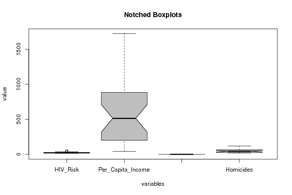
Title produced by software

Notched Boxplots

Date of computation

Tue, 24 Jan 2017 22:18:11 +0100

Cite this page as follows

Statistical Computations at FreeStatistics.org, Office for Research Development and Education, URL https://freestatistics.org/blog/index.php?v=date/2017/Jan/24/t1485292705fnwmh8674gt0wk9.htm/, Retrieved Tue, 14 May 2024 01:17:04 +0200

Statistical Computations at FreeStatistics.org, Office for Research Development and Education, URL https://freestatistics.org/blog/index.php?pk=, Retrieved Tue, 14 May 2024 01:17:04 +0200

QR Codes:

Paste this QR Code to cite your computation.

Original text written by user:

IsPrivate?

No (this computation is public)

User-defined keywords

Estimated Impact

Dataseries X:

Download CSV

Histogram

Boxplots

46.4 392 0.4 68.5
45.7 118 0.61 87.8
45.3 44 0.53 115.8
38.6 158 0.53 106.8
37.2 81 0.53 71.6
35 374 0.37 60.2
34 187 0.3 118.7
28.3 993 0.19 33.7
24.7 1723 0.12 27.2
24.7 287 0.2 62
24.4 970 0.19 24.9
22.7 885 0.12 22.9
22.3 200 0.53 65.7
21.7 575 0.14 21.6
21.6 688 0.34 32.4
21.3 48 0.69 108.7
21.2 572 0.49 38.6
20.8 239 0.42 46.7
20.3 244 0.48 56.5
18.9 472 0.25 44.4
18.8 134 0.52 47.4
18.6 633 0.19 21.7
18 295 0.44 55.7
17.6 906 0.24 27.1
17 1045 0.16 28.5
16.7 775 0.1 41.6
15.9 619 0.15 44.6
15.3 901 0.05 26.1
15 910 0.24 18.7
14.8 556 0.22 49.1

Summary of computational transaction
Raw Input	view raw input (R code)
Raw Output	view raw output of R engine
Computing time	1 seconds
R Server	Big Analytics Cloud Computing Center

\begin{tabular}{lllllllll}
\hline
Summary of computational transaction \tabularnewline
Raw Input view raw input (R code)  \tabularnewline
Raw Outputview raw output of R engine  \tabularnewline
Computing time1 seconds \tabularnewline
R ServerBig Analytics Cloud Computing Center \tabularnewline
\hline
\end{tabular}
%Source: https://freestatistics.org/blog/index.php?pk=&T=0

[TABLE]
[ROW]

Summary of computational transaction[/C][/ROW] [ROW]

Raw Input[/C]

view raw input (R code) [/C][/ROW] [ROW]

Raw Output[/C]

view raw output of R engine [/C][/ROW] [ROW]

Computing time[/C]

1 seconds[/C][/ROW] [ROW]

R Server[/C]

Big Analytics Cloud Computing Center[/C][/ROW] [/TABLE] Source: https://freestatistics.org/blog/index.php?pk=&T=0

Globally Unique Identifier (entire table): ba.freestatistics.org/blog/index.php?pk=&T=0

As an alternative you can also use a QR Code:

The GUIDs for individual cells are displayed in the table below:

Summary of computational transaction
Raw Input	view raw input (R code)
Raw Output	view raw output of R engine
Computing time	1 seconds
R Server	Big Analytics Cloud Computing Center

Boxplot statistics
Variable	lower whisker	lower hinge	median	upper hinge	upper whisker
HIV_Risk	14.8	18	21.45	28.3	38.6
Per_Capita_Income	44	200	514	885	1723
Prop_Population_on_Farms	0.05	0.19	0.275	0.49	0.69
Homicides	18.7	27.2	45.65	65.7	118.7

\begin{tabular}{lllllllll}
\hline
Boxplot statistics \tabularnewline
Variable & lower whisker & lower hinge & median & upper hinge & upper whisker \tabularnewline
HIV_Risk & 14.8 & 18 & 21.45 & 28.3 & 38.6 \tabularnewline
Per_Capita_Income & 44 & 200 & 514 & 885 & 1723 \tabularnewline
Prop_Population_on_Farms & 0.05 & 0.19 & 0.275 & 0.49 & 0.69 \tabularnewline
Homicides & 18.7 & 27.2 & 45.65 & 65.7 & 118.7 \tabularnewline
\hline
\end{tabular}
%Source: https://freestatistics.org/blog/index.php?pk=&T=1

[TABLE]
[ROW][C]Boxplot statistics[/C][/ROW]
[ROW][C]Variable[/C][C]lower whisker[/C][C]lower hinge[/C][C]median[/C][C]upper hinge[/C][C]upper whisker[/C][/ROW]
[ROW][C]HIV_Risk[/C][C]14.8[/C][C]18[/C][C]21.45[/C][C]28.3[/C][C]38.6[/C][/ROW]
[ROW][C]Per_Capita_Income[/C][C]44[/C][C]200[/C][C]514[/C][C]885[/C][C]1723[/C][/ROW]
[ROW][C]Prop_Population_on_Farms[/C][C]0.05[/C][C]0.19[/C][C]0.275[/C][C]0.49[/C][C]0.69[/C][/ROW]
[ROW][C]Homicides[/C][C]18.7[/C][C]27.2[/C][C]45.65[/C][C]65.7[/C][C]118.7[/C][/ROW]
[/TABLE]
Source: https://freestatistics.org/blog/index.php?pk=&T=1

Globally Unique Identifier (entire table): ba.freestatistics.org/blog/index.php?pk=&T=1

As an alternative you can also use a QR Code:

The GUIDs for individual cells are displayed in the table below:

Boxplot statistics
Variable	lower whisker	lower hinge	median	upper hinge	upper whisker
HIV_Risk	14.8	18	21.45	28.3	38.6
Per_Capita_Income	44	200	514	885	1723
Prop_Population_on_Farms	0.05	0.19	0.275	0.49	0.69
Homicides	18.7	27.2	45.65	65.7	118.7

Boxplot Notches
Variable	lower bound	median	upper bound
HIV_Risk	18.4787876997203	21.45	24.4212123002797
Per_Capita_Income	316.39995867072	514	711.60004132928
Prop_Population_on_Farms	0.188459835914184	0.275	0.361540164085816
Homicides	34.5440122756536	45.65	56.7559877243464

\begin{tabular}{lllllllll}
\hline
Boxplot Notches \tabularnewline
Variable & lower bound & median & upper bound \tabularnewline
HIV_Risk & 18.4787876997203 & 21.45 & 24.4212123002797 \tabularnewline
Per_Capita_Income & 316.39995867072 & 514 & 711.60004132928 \tabularnewline
Prop_Population_on_Farms & 0.188459835914184 & 0.275 & 0.361540164085816 \tabularnewline
Homicides & 34.5440122756536 & 45.65 & 56.7559877243464 \tabularnewline
\hline
\end{tabular}
%Source: https://freestatistics.org/blog/index.php?pk=&T=2

[TABLE]
[ROW][C]Boxplot Notches[/C][/ROW]
[ROW][C]Variable[/C][C]lower bound[/C][C]median[/C][C]upper bound[/C][/ROW]
[ROW][C]HIV_Risk[/C][C]18.4787876997203[/C][C]21.45[/C][C]24.4212123002797[/C][/ROW]
[ROW][C]Per_Capita_Income[/C][C]316.39995867072[/C][C]514[/C][C]711.60004132928[/C][/ROW]
[ROW][C]Prop_Population_on_Farms[/C][C]0.188459835914184[/C][C]0.275[/C][C]0.361540164085816[/C][/ROW]
[ROW][C]Homicides[/C][C]34.5440122756536[/C][C]45.65[/C][C]56.7559877243464[/C][/ROW]
[/TABLE]
Source: https://freestatistics.org/blog/index.php?pk=&T=2

Globally Unique Identifier (entire table): ba.freestatistics.org/blog/index.php?pk=&T=2

As an alternative you can also use a QR Code:

The GUIDs for individual cells are displayed in the table below:

Boxplot Notches
Variable	lower bound	median	upper bound
HIV_Risk	18.4787876997203	21.45	24.4212123002797
Per_Capita_Income	316.39995867072	514	711.60004132928
Prop_Population_on_Farms	0.188459835914184	0.275	0.361540164085816
Homicides	34.5440122756536	45.65	56.7559877243464

Figure 1

PNG link

Postscript link

PDF link

Parameters (Session):

par1 = 121248484848FALSE121101two.sidedgrey1111121212greygrey1111111111two.sidedtwo.sided12greytwo.sidedgrey1112greytwo.sidedgrey1111two.sidedtwo.sidedtwo.sidedtwo.sided111two.sidedtwo.sided12greypearson0.950.950.95greygrey ; par2 = -0.3-0.3-0.3-0.3-0.3-0.3Do not include Seasonal DummiesDo not include Seasonal DummiesDo not include Seasonal DummiesDo not include Seasonal Dummies0.95no2222nono222Do not include Seasonal DummiesDo not include Seasonal Dummies2222222Do not include Seasonal Dummies0.950.95SinglenoDo not include Seasonal Dummies0.95no22no0.99no22220.970.97Do not include Seasonal Dummies0.970.97222Do not include Seasonal Dummies0.950.95Doubleno-3-3-3nono ; par3 = 011000No Linear TrendNo Linear TrendNo Linear TrendNo Linear Trend1133Exact Pearson Chi-Squared by SimulationExact Pearson Chi-Squared by Simulation3Exact Pearson Chi-Squared by SimulationExact Pearson Chi-Squared by SimulationNo Linear TrendNo Linear TrendTRUE30,990,990,990.99Exact Pearson Chi-Squared by SimulationNo Linear Trend-3-3additiveNo Linear Trend113Exact Pearson Chi-Squared by Simulation1533Exact Pearson Chi-Squared by SimulationExact Pearson Chi-Squared by Simulation1919No Linear Trend191930.99Exact Pearson Chi-Squared by SimulationNo Linear Trend-3-3additive ; par4 = 001111FALSETRUETRUETRUEtwo.sidedtwo.sidedtwo.sidedtwo.sided12TRUETRUETRUETRUEtwo.sided1212 ; par5 = 121212121212pairedpairedpairedpairedpaired ; par6 = White NoiseWhite NoiseWhite NoiseWhite Noise3300000 ; par7 = 0.950.950.950.9510 ; par8 = 22 ; par9 = 10 ; par10 = FALSE ;

Parameters (R input):

par1 = grey ; par2 = no ;

R code (references can be found in the software module):

if(par2=='yes') {
z <- na.omit(as.data.frame(t(y)))
} else {
z <- as.data.frame(t(y))
}
bitmap(file='test1.png')
(r<-boxplot(z ,xlab=xlab,ylab=ylab,main=main,notch=TRUE,col=par1))
dev.off()
load(file='createtable')
a<-table.start()
a<-table.row.start(a)
a<-table.element(a,'Boxplot statistics',6,TRUE)
a<-table.row.end(a)
a<-table.row.start(a)
a<-table.element(a,'Variable',1,TRUE)
a<-table.element(a,'lower whisker',1,TRUE)
a<-table.element(a,'lower hinge',1,TRUE)
a<-table.element(a,'median',1,TRUE)
a<-table.element(a,'upper hinge',1,TRUE)
a<-table.element(a,'upper whisker',1,TRUE)
a<-table.row.end(a)
for (i in 1:length(y[,1]))
{
a<-table.row.start(a)
a<-table.element(a,dimnames(t(x))[[2]][i],1,TRUE)
for (j in 1:5)
{
a<-table.element(a,r$stats[j,i])
}
a<-table.row.end(a)
}
a<-table.end(a)
table.save(a,file='mytable.tab')
a<-table.start()
a<-table.row.start(a)
a<-table.element(a,'Boxplot Notches',4,TRUE)
a<-table.row.end(a)
a<-table.row.start(a)
a<-table.element(a,'Variable',1,TRUE)
a<-table.element(a,'lower bound',1,TRUE)
a<-table.element(a,'median',1,TRUE)
a<-table.element(a,'upper bound',1,TRUE)
a<-table.row.end(a)
for (i in 1:length(y[,1]))
{
a<-table.row.start(a)
a<-table.element(a,dimnames(t(x))[[2]][i],1,TRUE)
a<-table.element(a,r$conf[1,i])
a<-table.element(a,r$stats[3,i])
a<-table.element(a,r$conf[2,i])
a<-table.row.end(a)
}
a<-table.end(a)
table.save(a,file='mytable1.tab')

Free Statistics

Description of Statistical Computation

Tree of Dependent Computations

Dataset

Tables (Output of Computation)

Figures (Output of Computation)

Input Parameters & R Code