Free Statistics

of Irreproducible Research!

Author's title

Author*Unverified author*
R Software Modulerwasp_concentration.wasp
Title produced by softwareConcentration and Inequality
Date of computationTue, 30 Apr 2019 23:12:51 +0200
Cite this page as followsStatistical Computations at FreeStatistics.org, Office for Research Development and Education, URL https://freestatistics.org/blog/index.php?v=date/2019/Apr/30/t1556658850vdjrh41zy2azv04.htm/, Retrieved Mon, 29 Apr 2024 12:20:41 +0000
Statistical Computations at FreeStatistics.org, Office for Research Development and Education, URL https://freestatistics.org/blog/index.php?pk=318795, Retrieved Mon, 29 Apr 2024 12:20:41 +0000
QR Codes:

Original text written by user:
IsPrivate?No (this computation is public)
User-defined keywords
Estimated Impact112
Family? (F = Feedback message, R = changed R code, M = changed R Module, P = changed Parameters, D = changed Data)
-       [Concentration and Inequality] [Podaci završni] [2019-04-30 21:12:51] [d41d8cd98f00b204e9800998ecf8427e] [Current]
Feedback Forum

Post a new message
Dataseries X:
39434749
7559163
5366695
2445397
931854
1439251
445055
1234615
1327803
962431
321421
99211
1851
233153
132771


Summary of computational transaction
Raw Input view raw input (R code)
Raw Outputview raw output of R engine
Computing time1 seconds
R ServerBig Analytics Cloud Computing Center

\begin{tabular}{lllllllll}
\hline
Summary of computational transaction \tabularnewline
Raw Input view raw input (R code)  \tabularnewline
Raw Outputview raw output of R engine  \tabularnewline
Computing time1 seconds \tabularnewline
R ServerBig Analytics Cloud Computing Center \tabularnewline
\hline
\end{tabular}
%Source: https://freestatistics.org/blog/index.php?pk=318795&T=0

[TABLE]
[ROW]
Summary of computational transaction[/C][/ROW] [ROW]Raw Input[/C] view raw input (R code) [/C][/ROW] [ROW]Raw Output[/C]view raw output of R engine [/C][/ROW] [ROW]Computing time[/C]1 seconds[/C][/ROW] [ROW]R Server[/C]Big Analytics Cloud Computing Center[/C][/ROW] [/TABLE] Source: https://freestatistics.org/blog/index.php?pk=318795&T=0

Globally Unique Identifier (entire table): ba.freestatistics.org/blog/index.php?pk=318795&T=0

As an alternative you can also use a QR Code:  

The GUIDs for individual cells are displayed in the table below:

Summary of computational transaction
Raw Input view raw input (R code)
Raw Outputview raw output of R engine
Computing time1 seconds
R ServerBig Analytics Cloud Computing Center


Concentration - Ungrouped Data
MeasureValue
Number of Categories15
Maximum Entropy2.70805020110221
Entropy1.36696646468234
Normalised Entropy0.504778849419395
Max. Entropy - Entropy1.34108373641987
Theil Entropy Index1.34108373641987
Exponential Index0.254878972361101
Herfindahl0.431324295296049
Normalised Herfindahl0.39070460210291
Rosenbluth0.299826861146342
Gini0.777649452714887
Concentration0.833195842194522
Ricci-Schutz (Pietra)0.645406505679626
Atkinson0.536176926290531
KolmInf
Coefficient of Variation2.33877412963303
Squared Coefficient of Variation5.46986442944074

\begin{tabular}{lllllllll}
\hline
Concentration - Ungrouped Data \tabularnewline
Measure & Value \tabularnewline
Number of Categories & 15 \tabularnewline
Maximum Entropy & 2.70805020110221 \tabularnewline
Entropy & 1.36696646468234 \tabularnewline
Normalised Entropy & 0.504778849419395 \tabularnewline
Max. Entropy - Entropy & 1.34108373641987 \tabularnewline
Theil Entropy Index & 1.34108373641987 \tabularnewline
Exponential Index & 0.254878972361101 \tabularnewline
Herfindahl & 0.431324295296049 \tabularnewline
Normalised Herfindahl & 0.39070460210291 \tabularnewline
Rosenbluth & 0.299826861146342 \tabularnewline
Gini & 0.777649452714887 \tabularnewline
Concentration & 0.833195842194522 \tabularnewline
Ricci-Schutz (Pietra) & 0.645406505679626 \tabularnewline
Atkinson & 0.536176926290531 \tabularnewline
Kolm & Inf \tabularnewline
Coefficient of Variation & 2.33877412963303 \tabularnewline
Squared Coefficient of Variation & 5.46986442944074 \tabularnewline
\hline
\end{tabular}
%Source: https://freestatistics.org/blog/index.php?pk=318795&T=1

[TABLE]
[ROW][C]Concentration - Ungrouped Data[/C][/ROW]
[ROW][C]Measure[/C][C]Value[/C][/ROW]
[ROW][C]Number of Categories[/C][C]15[/C][/ROW]
[ROW][C]Maximum Entropy[/C][C]2.70805020110221[/C][/ROW]
[ROW][C]Entropy[/C][C]1.36696646468234[/C][/ROW]
[ROW][C]Normalised Entropy[/C][C]0.504778849419395[/C][/ROW]
[ROW][C]Max. Entropy - Entropy[/C][C]1.34108373641987[/C][/ROW]
[ROW][C]Theil Entropy Index[/C][C]1.34108373641987[/C][/ROW]
[ROW][C]Exponential Index[/C][C]0.254878972361101[/C][/ROW]
[ROW][C]Herfindahl[/C][C]0.431324295296049[/C][/ROW]
[ROW][C]Normalised Herfindahl[/C][C]0.39070460210291[/C][/ROW]
[ROW][C]Rosenbluth[/C][C]0.299826861146342[/C][/ROW]
[ROW][C]Gini[/C][C]0.777649452714887[/C][/ROW]
[ROW][C]Concentration[/C][C]0.833195842194522[/C][/ROW]
[ROW][C]Ricci-Schutz (Pietra)[/C][C]0.645406505679626[/C][/ROW]
[ROW][C]Atkinson[/C][C]0.536176926290531[/C][/ROW]
[ROW][C]Kolm[/C][C]Inf[/C][/ROW]
[ROW][C]Coefficient of Variation[/C][C]2.33877412963303[/C][/ROW]
[ROW][C]Squared Coefficient of Variation[/C][C]5.46986442944074[/C][/ROW]
[/TABLE]
Source: https://freestatistics.org/blog/index.php?pk=318795&T=1

Globally Unique Identifier (entire table): ba.freestatistics.org/blog/index.php?pk=318795&T=1

As an alternative you can also use a QR Code:  

The GUIDs for individual cells are displayed in the table below:

Concentration - Ungrouped Data
MeasureValue
Number of Categories15
Maximum Entropy2.70805020110221
Entropy1.36696646468234
Normalised Entropy0.504778849419395
Max. Entropy - Entropy1.34108373641987
Theil Entropy Index1.34108373641987
Exponential Index0.254878972361101
Herfindahl0.431324295296049
Normalised Herfindahl0.39070460210291
Rosenbluth0.299826861146342
Gini0.777649452714887
Concentration0.833195842194522
Ricci-Schutz (Pietra)0.645406505679626
Atkinson0.536176926290531
KolmInf
Coefficient of Variation2.33877412963303
Squared Coefficient of Variation5.46986442944074


Parameters (Session):
Parameters (R input):
R code (references can be found in the software module):
library(ineq)
my_minimum <- min(x)
if(my_minimum < 0) {
stop('Negative values are not allowed.')
}
myLength <- length(x)
myMaximumEntropy <- log(myLength)
mySum <- sum(x)
myProportion <- x/mySum
myEntropy <- -sum(myProportion * log(myProportion))
myNormalizedEntropy <- myEntropy / myMaximumEntropy
myDifference <- myMaximumEntropy - myEntropy
myTheilEntropyIndex <- entropy(x,parameter=1,na.rm=T)
myExponentialIndex <- exp(-myEntropy)
myHerfindahlMeasure <- sum(myProportion^2)
myHerfindahl <- conc(x,type='Herfindahl',na.rm=T)
myRosenbluth <- conc(x,type='Rosenbluth',na.rm=T)
myNormalizedHerfindahlMeasure <- (myHerfindahlMeasure - 1/myLength) / (1 - 1/myLength)
myGini <- Gini(x,na.rm=T)
myConcentrationCoefficient <- myLength/(myLength -1)*myGini
myRS <- RS(x,na.rm=T)
myAtkinson <- Atkinson(x,na.rm=T)
myKolm <- Kolm(x,na.rm=T)
myCoefficientOfVariation <- var.coeff(x,square=F,na.rm=T)
mySquaredCoefficientOfVariation <- var.coeff(x,square=T,na.rm=T)
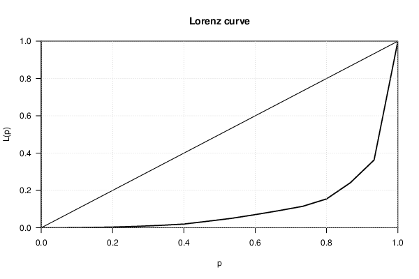
bitmap(file='plot1.png')
plot(Lc(x))
grid()
dev.off()
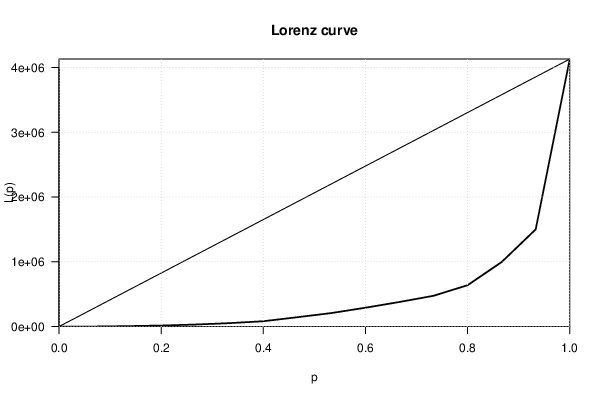
bitmap(file='plot2.png')
plot(Lc(x),general=T)
grid()
dev.off()
load(file='createtable')
a<-table.start()
a<-table.row.start(a)
a<-table.element(a,'Concentration - Ungrouped Data',2,TRUE)
a<-table.row.end(a)
a<-table.row.start(a)
a<-table.element(a,'Measure',header=TRUE)
a<-table.element(a,'Value',header=TRUE)
a<-table.row.end(a)
a<-table.row.start(a)
a<-table.element(a,'Number of Categories',header=F)
a<-table.element(a,myLength,header=F)
a<-table.row.end(a)
a<-table.row.start(a)
a<-table.element(a,'Maximum Entropy',header=F)
a<-table.element(a,myMaximumEntropy,header=F)
a<-table.row.end(a)
a<-table.row.start(a)
a<-table.element(a,'Entropy',header=F)
a<-table.element(a,myEntropy,header=F)
a<-table.row.end(a)
a<-table.row.start(a)
a<-table.element(a,'Normalised Entropy',header=F)
a<-table.element(a,myNormalizedEntropy,header=F)
a<-table.row.end(a)
a<-table.row.start(a)
a<-table.element(a,'Max. Entropy - Entropy',header=F)
a<-table.element(a,myDifference,header=F)
a<-table.row.end(a)
a<-table.row.start(a)
a<-table.element(a,'Theil Entropy Index',header=F)
a<-table.element(a,myTheilEntropyIndex,header=F)
a<-table.row.end(a)
a<-table.row.start(a)
a<-table.element(a,'Exponential Index',header=F)
a<-table.element(a,myExponentialIndex,header=F)
a<-table.row.end(a)
a<-table.row.start(a)
a<-table.element(a,'Herfindahl',header=F)
a<-table.element(a,myHerfindahl,header=F)
a<-table.row.end(a)
a<-table.row.start(a)
a<-table.element(a,'Normalised Herfindahl',header=F)
a<-table.element(a,myNormalizedHerfindahlMeasure,header=F)
a<-table.row.end(a)
a<-table.row.start(a)
a<-table.element(a,'Rosenbluth',header=F)
a<-table.element(a,myRosenbluth,header=F)
a<-table.row.end(a)
a<-table.row.start(a)
a<-table.element(a,'Gini',header=F)
a<-table.element(a,myGini,header=F)
a<-table.row.end(a)
a<-table.row.start(a)
a<-table.element(a,'Concentration',header=F)
a<-table.element(a,myConcentrationCoefficient,header=F)
a<-table.row.end(a)
a<-table.row.start(a)
a<-table.element(a,'Ricci-Schutz (Pietra)',header=F)
a<-table.element(a,myRS,header=F)
a<-table.row.end(a)
a<-table.row.start(a)
a<-table.element(a,'Atkinson',header=F)
a<-table.element(a,myAtkinson,header=F)
a<-table.row.end(a)
a<-table.row.start(a)
a<-table.element(a,'Kolm',header=F)
a<-table.element(a,myKolm,header=F)
a<-table.row.end(a)
a<-table.row.start(a)
a<-table.element(a,'Coefficient of Variation',header=F)
a<-table.element(a,myCoefficientOfVariation,header=F)
a<-table.row.end(a)
a<-table.row.start(a)
a<-table.element(a,'Squared Coefficient of Variation',header=F)
a<-table.element(a,mySquaredCoefficientOfVariation,header=F)
a<-table.row.end(a)
a<-table.end(a)
table.save(a,file='mytable.tab')