Free Statistics
of Irreproducible Research!
Description of Statistical Computation | ||||||||||||||||||||||||||||||||||||||||||||||||||||||||||||||||||||||||||||||||||||||||||||||||||||||||||||||||||||||||||||||||||||||||||||||||||||||||||||||||||||||||||||||||||||||||||||
|---|---|---|---|---|---|---|---|---|---|---|---|---|---|---|---|---|---|---|---|---|---|---|---|---|---|---|---|---|---|---|---|---|---|---|---|---|---|---|---|---|---|---|---|---|---|---|---|---|---|---|---|---|---|---|---|---|---|---|---|---|---|---|---|---|---|---|---|---|---|---|---|---|---|---|---|---|---|---|---|---|---|---|---|---|---|---|---|---|---|---|---|---|---|---|---|---|---|---|---|---|---|---|---|---|---|---|---|---|---|---|---|---|---|---|---|---|---|---|---|---|---|---|---|---|---|---|---|---|---|---|---|---|---|---|---|---|---|---|---|---|---|---|---|---|---|---|---|---|---|---|---|---|---|---|---|---|---|---|---|---|---|---|---|---|---|---|---|---|---|---|---|---|---|---|---|---|---|---|---|---|---|---|---|---|---|---|---|---|
| Author's title | ||||||||||||||||||||||||||||||||||||||||||||||||||||||||||||||||||||||||||||||||||||||||||||||||||||||||||||||||||||||||||||||||||||||||||||||||||||||||||||||||||||||||||||||||||||||||||||
| Author | *The author of this computation has been verified* | |||||||||||||||||||||||||||||||||||||||||||||||||||||||||||||||||||||||||||||||||||||||||||||||||||||||||||||||||||||||||||||||||||||||||||||||||||||||||||||||||||||||||||||||||||||||||||
| R Software Module | rwasp_Simple Regression Y ~ X.wasp | |||||||||||||||||||||||||||||||||||||||||||||||||||||||||||||||||||||||||||||||||||||||||||||||||||||||||||||||||||||||||||||||||||||||||||||||||||||||||||||||||||||||||||||||||||||||||||
| Title produced by software | Simple Linear Regression | |||||||||||||||||||||||||||||||||||||||||||||||||||||||||||||||||||||||||||||||||||||||||||||||||||||||||||||||||||||||||||||||||||||||||||||||||||||||||||||||||||||||||||||||||||||||||||
| Date of computation | Sat, 19 Jan 2019 15:29:20 +0100 | |||||||||||||||||||||||||||||||||||||||||||||||||||||||||||||||||||||||||||||||||||||||||||||||||||||||||||||||||||||||||||||||||||||||||||||||||||||||||||||||||||||||||||||||||||||||||||
| Cite this page as follows | Statistical Computations at FreeStatistics.org, Office for Research Development and Education, URL https://freestatistics.org/blog/index.php?v=date/2019/Jan/19/t15479081905vsap4klaz59fz8.htm/, Retrieved Tue, 07 May 2024 22:52:57 +0000 | |||||||||||||||||||||||||||||||||||||||||||||||||||||||||||||||||||||||||||||||||||||||||||||||||||||||||||||||||||||||||||||||||||||||||||||||||||||||||||||||||||||||||||||||||||||||||||
| Statistical Computations at FreeStatistics.org, Office for Research Development and Education, URL https://freestatistics.org/blog/index.php?pk=316342, Retrieved Tue, 07 May 2024 22:52:57 +0000 | ||||||||||||||||||||||||||||||||||||||||||||||||||||||||||||||||||||||||||||||||||||||||||||||||||||||||||||||||||||||||||||||||||||||||||||||||||||||||||||||||||||||||||||||||||||||||||||
| QR Codes: | ||||||||||||||||||||||||||||||||||||||||||||||||||||||||||||||||||||||||||||||||||||||||||||||||||||||||||||||||||||||||||||||||||||||||||||||||||||||||||||||||||||||||||||||||||||||||||||
|
| ||||||||||||||||||||||||||||||||||||||||||||||||||||||||||||||||||||||||||||||||||||||||||||||||||||||||||||||||||||||||||||||||||||||||||||||||||||||||||||||||||||||||||||||||||||||||||||
| Original text written by user: | ||||||||||||||||||||||||||||||||||||||||||||||||||||||||||||||||||||||||||||||||||||||||||||||||||||||||||||||||||||||||||||||||||||||||||||||||||||||||||||||||||||||||||||||||||||||||||||
| IsPrivate? | No (this computation is public) | |||||||||||||||||||||||||||||||||||||||||||||||||||||||||||||||||||||||||||||||||||||||||||||||||||||||||||||||||||||||||||||||||||||||||||||||||||||||||||||||||||||||||||||||||||||||||||
| User-defined keywords | ||||||||||||||||||||||||||||||||||||||||||||||||||||||||||||||||||||||||||||||||||||||||||||||||||||||||||||||||||||||||||||||||||||||||||||||||||||||||||||||||||||||||||||||||||||||||||||
| Estimated Impact | 78 | |||||||||||||||||||||||||||||||||||||||||||||||||||||||||||||||||||||||||||||||||||||||||||||||||||||||||||||||||||||||||||||||||||||||||||||||||||||||||||||||||||||||||||||||||||||||||||
Tree of Dependent Computations | ||||||||||||||||||||||||||||||||||||||||||||||||||||||||||||||||||||||||||||||||||||||||||||||||||||||||||||||||||||||||||||||||||||||||||||||||||||||||||||||||||||||||||||||||||||||||||||
| Family? (F = Feedback message, R = changed R code, M = changed R Module, P = changed Parameters, D = changed Data) | ||||||||||||||||||||||||||||||||||||||||||||||||||||||||||||||||||||||||||||||||||||||||||||||||||||||||||||||||||||||||||||||||||||||||||||||||||||||||||||||||||||||||||||||||||||||||||||
| - [Simple Linear Regression] [] [2019-01-19 14:29:20] [98fe8ff2db3eaf59b568f46d4a014cb6] [Current] | ||||||||||||||||||||||||||||||||||||||||||||||||||||||||||||||||||||||||||||||||||||||||||||||||||||||||||||||||||||||||||||||||||||||||||||||||||||||||||||||||||||||||||||||||||||||||||||
| Feedback Forum | ||||||||||||||||||||||||||||||||||||||||||||||||||||||||||||||||||||||||||||||||||||||||||||||||||||||||||||||||||||||||||||||||||||||||||||||||||||||||||||||||||||||||||||||||||||||||||||
Post a new message | ||||||||||||||||||||||||||||||||||||||||||||||||||||||||||||||||||||||||||||||||||||||||||||||||||||||||||||||||||||||||||||||||||||||||||||||||||||||||||||||||||||||||||||||||||||||||||||
Dataset | ||||||||||||||||||||||||||||||||||||||||||||||||||||||||||||||||||||||||||||||||||||||||||||||||||||||||||||||||||||||||||||||||||||||||||||||||||||||||||||||||||||||||||||||||||||||||||||
| Dataseries X: | ||||||||||||||||||||||||||||||||||||||||||||||||||||||||||||||||||||||||||||||||||||||||||||||||||||||||||||||||||||||||||||||||||||||||||||||||||||||||||||||||||||||||||||||||||||||||||||
1 0.5 0.67 0.67 0 0.5 2011 1 0 149 0.89 0.5 0.83 0.33 0.5 1 2011 1 1 139 0.89 0.4 1 0.67 0 1 2011 1 0 148 0.89 0.5 0.83 0 0 0 2011 1 1 158 0.89 0.7 0.67 0 1 1 2011 1 1 128 0.78 0.3 0 0 0.5 0.5 2011 1 1 224 0.89 0.4 0.83 0.67 0.5 0 2011 1 0 159 1 0.4 0.5 0.67 1 1 2011 1 1 105 0.89 0.7 0.83 0 0.5 0 2011 1 1 159 0.78 0.6 0.33 0.67 0.5 0.5 2011 1 1 167 1 0.6 0.5 1 0 0.5 2011 1 1 165 0.78 0.2 0.67 0 0.5 0.5 2011 1 1 159 0.89 0.4 1 0 0.5 0.5 2011 1 1 119 0.89 0.4 0.5 0.67 0 1 2011 1 0 176 0.89 0.5 0.67 0.33 0 0 2011 1 0 54 0.89 0.3 0.17 0.67 0 0.5 2011 0 0 91 0.89 0.4 0.83 0.33 0.5 0.5 2011 1 1 163 0.67 0.7 0.67 0.33 0.5 1 2011 1 0 124 1 0.5 0.67 0.33 0 1 2011 0 1 137 0.78 0.2 0.67 0 0 1 2011 1 0 121 0.78 0.3 0.5 0.67 0 0.5 2011 1 1 153 0.89 0.6 1 0.33 0 1 2011 1 1 148 0.78 0.6 0.83 0.33 0 1 2011 1 0 221 0.89 0.2 0.83 0.33 0 1 2011 1 1 188 0.89 0.7 1 0.67 1 0 2011 1 1 149 0.33 0.2 0.67 0 0 0 2011 1 1 244 1 1 1 0.33 1 1 2011 0 1 148 0.89 0.4 0.83 0.67 0 0.5 2011 0 0 92 0.89 0.4 1 1 0 1 2011 1 1 150 0.67 0.2 0.83 0.67 0 0.5 2011 1 0 153 0.56 0.4 0.67 0.33 0 1 2011 1 0 94 0.89 0.4 0.67 0 0.5 1 2011 1 0 156 0.89 0.7 1 0.67 0.5 0.5 2011 1 1 132 1 0.2 0.67 0.67 0 0.5 2011 1 1 161 0.78 0.6 1 1 0 0.5 2011 1 1 105 0.78 0.3 1 1 0.5 0.5 2011 1 1 97 0.33 0.3 0.5 0.33 0 0 2011 1 0 151 0.78 0.2 0.67 0 0.5 0 2011 0 1 131 0.89 0.5 0.83 0.67 0.5 0.5 2011 1 1 166 0.89 0.7 1 0.67 0.5 1 2011 1 0 157 0.78 0.6 1 0.67 0.5 0.5 2011 1 1 111 0.89 0.4 1 0.67 0.5 1 2011 1 1 145 0.89 0.6 1 0.33 0.5 1 2011 1 1 162 1 0.4 1 1 0 1 2011 1 1 163 0.67 0.3 0.83 0.67 0 1 2011 0 1 59 1 0.5 0.83 0.67 0.5 0.5 2011 1 0 187 0.89 0.2 0.5 0 0 1 2011 1 1 109 0.89 0.3 0.83 0 0.5 1 2011 0 1 90 0.89 0.5 0.17 0 0 1 2011 1 0 105 0.78 0.7 0.83 1 0.5 1 2011 0 1 83 0.89 0.4 1 0.67 1 0.5 2011 0 1 116 0.78 0.3 1 0 0 0.5 2011 0 1 42 0.78 0.2 0.67 0.67 1 1 2011 1 1 148 1 0.5 1 0 0 0.5 2011 0 1 155 0.78 0.4 1 0 0.5 0 2011 1 1 125 1 0.6 1 0.67 1 1 2011 1 1 116 0.78 0.4 0.83 1 0 1 2011 0 0 128 0.67 0.4 0.33 0 0 0.5 2011 1 1 138 0.33 0.2 0.33 0.33 0 0 2011 0 0 49 1 0.9 1 0.67 0.5 1 2011 0 1 96 1 0.8 1 0.67 1 0.5 2011 1 1 164 0.78 0.8 0.83 0 0.5 1 2011 1 0 162 0.67 0.3 1 1 0.5 1 2011 1 0 99 1 0.2 0.83 0.67 0 0.5 2011 1 1 202 0.89 0.4 0.67 0 0.5 1 2011 1 0 186 0.89 0.2 0.83 1 0 1 2011 0 1 66 0.78 0.2 0.67 0.67 0.5 1 2011 1 0 183 1 0.1 0.83 0.67 0 1 2011 1 1 214 0.56 0.4 0.67 1 0.5 0 2011 1 1 188 0.67 0.5 1 0 0.5 0.5 2011 0 0 104 0.89 0.8 0.83 0.33 0.5 1 2011 1 0 177 0.89 0.4 0.67 0.67 0 0.5 2011 1 0 126 0.89 0.6 0.83 0.33 0.5 0.5 2011 0 0 76 0.89 0.5 0.83 0.67 0.5 1 2011 0 1 99 0.78 0.3 0.67 0 0 0 2011 1 0 139 1 0.4 0.33 0 0.5 0 2011 1 0 162 1 0.6 0.83 0.67 0.5 0.5 2011 0 1 108 0.89 0.4 1 0.33 0 0.5 2011 1 0 159 0.44 0.3 0.83 0 0 0 2011 0 0 74 0.78 0.8 0.83 0 1 1 2011 1 1 110 0.89 0.6 0.5 0.33 1 1 2011 0 0 96 0.67 0.3 0.5 0 0 0 2011 0 0 116 0.78 0.5 0.83 0.67 0.5 1 2011 0 0 87 0.78 0.4 1 0.33 0 1 2011 0 1 97 0.33 0.3 0.33 0.67 0 0 2011 0 0 127 0.89 0.7 1 0.33 0 0.5 2011 0 1 106 0.89 0.2 0.67 0.33 0.5 0.5 2011 0 1 80 0.89 0.4 0.83 1 0 1 2011 0 0 74 0.89 0.6 1 0.67 0.5 0.5 2011 0 0 91 0.56 0.6 0.83 0 0 1 2011 0 0 133 0.67 0.6 0.83 0.67 0.5 0.5 2011 0 1 74 0.67 0.4 1 0.33 0.5 1 2011 0 1 114 0.78 0.6 0.83 0 0 1 2011 0 1 140 0.78 0.5 1 0.33 0.5 1 2011 0 0 95 0.78 0.5 0.83 0 0 1 2011 0 1 98 0.89 0.6 0.67 0 0 1 2011 0 0 121 1 0.8 0.83 0.33 0.5 1 2011 0 1 126 0.89 0.5 0.83 0.67 1 0.5 2011 0 1 98 0.89 0.6 0.83 0.67 0.5 1 2011 0 1 95 0.78 0.4 0.83 0.67 0.5 1 2011 0 1 110 1 0.3 0.67 0.67 0.5 1 2011 0 1 70 0.78 0.3 0.83 1 0 0.5 2011 0 0 102 0.67 0.2 0 0 0 0 2011 0 1 86 0.78 0.4 0.83 0 0 0.5 2011 0 1 130 0.89 0.5 1 0 0 0.5 2011 0 1 96 0.67 0.3 0.17 0 0.5 0 2011 0 0 102 0.22 0.4 0.17 0 0.5 0 2011 0 0 100 0.44 0.5 0.5 1 0 0 2011 0 0 94 0.89 0.3 0.5 0.67 0 1 2011 0 0 52 0.67 0.5 1 0 0 0.5 2011 0 0 98 0.89 0.4 0.67 0.67 0 0.5 2011 0 0 118 0.67 0.4 0.83 0.67 0 1 2011 0 1 99 0.78 0.6 1 0 1 1 2012 1 1 48 0.78 0.3 1 0.67 1 1 2012 1 1 50 0.78 0.4 1 0.33 1 0.5 2012 1 1 150 1 0.3 1 1 1 1 2012 1 1 154 0.78 1 1 1 1 1 2012 0 0 109 0.67 0.4 1 0 0 0.5 2012 0 1 68 0.89 0.8 0.83 1 0.5 1 2012 1 1 194 0.89 0.3 1 0.67 1 1 2012 1 0 158 1 0.5 0.83 0.67 0 1 2012 1 1 159 0.78 0.4 1 0 0 0.5 2012 1 0 67 0.67 0.3 0.83 0.67 0 1 2012 1 0 147 0.89 0.5 0.83 1 0 1 2012 1 1 39 0.67 0.3 1 0.67 0 1 2012 1 1 100 0.67 0.3 0.67 0 0 1 2012 1 1 111 1 0.4 0.83 0 0 1 2012 1 1 138 0.67 0.3 1 0 0 0.5 2012 1 1 101 1 0.6 1 0.33 0.5 0.5 2012 0 1 131 0.89 0.6 0.83 0.67 1 1 2012 1 1 101 0.89 0.4 1 1 1 1 2012 1 1 114 1 0.4 1 0 0 0 2012 1 0 165 0.67 0.4 1 0.67 0 0.5 2012 1 1 114 0.44 0.3 0.67 0.67 0.5 1 2012 1 1 111 0.89 0.2 1 0.33 1 0 2012 1 1 75 0.56 0.5 0.83 0.67 0 1 2012 1 1 82 0.78 0.4 1 0.67 1 1 2012 1 1 121 1 0.4 1 0.67 0 0 2012 1 1 32 1 0.4 0.83 0.67 0 1 2012 1 0 150 0.89 0.3 0.67 0.67 0.5 0.5 2012 1 1 117 0.67 0.4 0.83 0.67 1 0.5 2012 0 1 71 0.89 0.2 1 0.33 0.5 1 2012 1 1 165 0.33 0 0 0 0 0 2012 1 1 154 0.89 0.4 1 0.67 0.5 1 2012 1 1 126 0.78 0.6 1 0 1 1 2012 1 0 149 1 0.4 0.67 0.67 0 0.5 2012 1 0 145 0.44 0.4 1 0 0 0.5 2012 1 1 120 0.67 0.4 0.83 0 0.5 0 2012 1 0 109 0.33 0.2 0.17 0 0.5 0 2012 1 0 132 0.89 0.4 0.83 1 1 1 2012 1 1 172 0.89 0.3 0.83 0 0 0.5 2012 1 0 169 1 0.6 0.83 0.67 1 0 2012 1 1 114 0.89 0.6 0.83 1 0 1 2012 1 1 156 0.89 0.4 0.83 0 0 1 2012 1 0 172 1 0.5 1 0.67 1 0.5 2012 0 1 68 0.89 0.4 0.83 0 0.5 1 2012 0 1 89 1 0.6 1 1 1 1 2012 1 1 167 0.78 0.6 0.83 0.67 0.5 1 2012 1 0 113 0.78 0.9 1 0.67 0.5 1 2012 0 0 115 0.67 0.4 0.83 0.67 0.5 0 2012 0 0 78 0.89 0.8 1 1 0.5 1 2012 0 0 118 0.67 0.5 0.83 1 0 1 2012 0 1 87 0.78 0.4 0.83 1 0 0 2012 1 0 173 0.89 0.4 1 0.67 1 0.5 2012 1 1 2 0.89 0.7 1 1 1 0.5 2012 0 0 162 0.78 0.4 1 0.33 1 1 2012 0 1 49 1 0.8 1 0.67 0.5 1 2012 0 0 122 1 0.4 1 1 1 0.5 2012 0 1 96 1 0.3 1 0.67 0 0.5 2012 0 0 100 0.67 0.5 1 0.67 0.5 1 2012 0 0 82 0.89 0.8 1 0.67 1 1 2012 0 1 100 1 0.4 0.83 0.33 0 0.5 2012 0 0 115 1 1 1 1 0.5 0 2012 0 1 141 0.89 0.5 1 0.67 1 1 2012 1 1 165 0.89 0.5 1 0.67 1 1 2012 1 1 165 0.89 0.3 1 0.33 0 1 2012 0 1 110 0.89 0.3 0.83 0.33 0.5 1 2012 1 1 118 0.89 0.3 0.5 0 0 1 2012 1 0 158 1 0.4 0.67 0.33 0.5 0.5 2012 0 1 146 0.67 0.5 1 0.33 0 1 2012 1 0 49 1 0.5 0.67 0.67 0.5 1 2012 0 0 90 0.89 0.4 1 0 0 0 2012 0 0 121 0.89 0.7 1 1 0.5 0 2012 1 1 155 0.89 0.5 0.5 0.33 0 0.5 2012 0 0 104 0.89 0.4 0.67 0.33 1 0 2012 0 1 147 1 0.7 0.67 1 0 1 2012 0 0 110 1 0.7 0.67 1 0 1 2012 0 0 108 1 0.7 0.67 1 0 1 2012 0 0 113 0.89 0.7 0.67 1 0 1 2012 0 0 115 0.89 0.7 0.67 0 0 0 2012 0 1 61 0.89 0.7 1 0.67 0.5 1 2012 0 1 60 0.33 0.1 0.67 0.33 0.5 0 2012 0 1 109 0.67 0.2 0.67 0.67 0.5 1 2012 0 1 68 0.56 0.3 0.33 0.33 0 1 2012 0 0 111 0.44 0.6 0.83 0.33 0 0.5 2012 0 0 77 1 0.8 1 1 1 1 2012 0 1 73 0.89 0.8 1 0.33 0.5 0.5 2012 1 0 151 0.33 0 0.17 0 0 0 2012 0 0 89 0.67 0.3 0.67 0.33 0 1 2012 0 0 78 0.67 0.6 0.83 0.33 0.5 1 2012 0 0 110 1 0.5 0.83 0.67 0 1 2012 1 1 220 0.78 0.7 1 0.33 0 0.5 2012 0 1 65 0.67 0.3 0.83 0 0.5 1 2012 1 0 141 1 0.3 1 0.67 0 0 2012 0 0 117 0.78 0.4 1 0.67 0 0.5 2012 1 1 122 0.89 0.4 0.83 1 0 1 2012 0 0 63 0.89 0.1 0.83 0 0 1 2012 1 1 44 0.89 0.5 1 0.67 0 1 2012 0 1 52 0 0 0 0 0 0 2012 0 0 131 0.67 0.4 1 0.33 0.5 0 2012 0 1 101 1 0.6 0.83 0.67 1 0.5 2012 0 1 42 1 0.4 1 0.33 0.5 1 2012 1 1 152 0.67 0.1 0.33 0 0.5 1 2012 1 0 107 0.89 0.3 0.83 0 0 1 2012 0 0 77 0.89 0.7 0.83 0.67 0 1 2012 1 0 154 0.56 0.3 0.17 0 0 1 2012 1 1 103 0.67 0.5 0.83 0.33 0.5 0 2012 0 1 96 1 0.3 0.83 0.67 1 1 2012 1 1 175 1 0.6 0.67 0.67 0.5 1 2012 0 1 57 1 0.9 1 1 0 1 2012 0 0 112 0.67 0.4 0.83 0 0.5 1 2012 1 0 143 0.44 0.3 1 0 0.5 0.5 2012 0 0 49 0.89 0.9 1 0.67 1 1 2012 1 1 110 0.44 0.5 1 0 0.5 0 2012 1 1 131 0.56 0.3 1 1 0.5 0.5 2012 1 0 167 0.89 0.6 0.83 0.67 0 0.5 2012 0 0 56 0.67 0.2 1 0.33 0 0.5 2012 1 0 137 0.89 0.4 0.83 1 0.5 1 2012 0 1 86 1 0.5 0.83 0.67 0.5 0.5 2012 1 1 121 0.78 0.4 0.83 0.67 0 0.5 2012 1 0 149 0.44 0 0 0 0 0 2012 1 0 168 0.89 0.2 1 0.33 0.5 1 2012 1 0 140 0.89 0.5 1 0.67 0.5 1 2012 0 1 88 0.89 0.3 1 0.67 0 0.5 2012 1 1 168 0.44 0 0 0 0 0 2012 1 1 94 1 0.5 0.83 1 0 1 2012 1 1 51 0.89 0.6 0.83 0.33 0 1 2012 0 0 48 0.67 0.3 0.83 0 0.5 0.5 2012 1 1 145 0.33 0 0 0 0 0 2012 1 1 66 0.78 0.3 0.67 0 0.5 0 2012 0 1 85 0.89 0.5 1 0.67 0.5 1 2012 1 0 109 0.78 0.4 0.67 0 0 1 2012 0 0 63 0.78 0.5 0.83 0.67 0 0.5 2012 0 1 102 0.89 0.7 1 1 1 0.5 2012 0 0 162 0.78 0.8 1 0.67 0.5 1 2012 0 1 86 0.78 0.6 1 0.33 0.5 1 2012 0 1 114 0.67 0.4 0.83 0.33 0 0.5 2012 1 0 164 0.89 0.5 0.83 0.33 0.5 0 2012 1 1 119 0.89 0.5 1 0 0.5 1 2012 1 0 126 0.78 0.3 1 0.33 0 1 2012 1 1 132 1 0.6 1 0 0.5 1 2012 1 1 142 1 0.3 0.67 0.67 0 0.5 2012 1 0 83 0.78 0.6 0.83 1 0.5 0.5 2012 0 1 94 0.78 0.3 0.33 0.33 0 1 2012 0 0 81 0.89 0.7 1 0.67 1 1 2012 1 1 166 0.89 0.7 1 1 0 1 2012 0 0 110 0.67 0.6 0.67 1 0.5 1 2012 0 1 64 1 0.5 1 0.33 0.5 0 2012 1 0 93 0.67 0.5 0.83 0.33 0 0.5 2012 0 0 104 0.56 0.4 0.67 0 0 1 2012 0 1 105 0.78 0.4 1 0.33 1 1 2012 0 1 49 1 0.7 1 1 0 1 2012 0 0 88 0.67 0.2 0.17 0 0.5 0 2012 0 1 95 0.78 0.5 0.83 0.67 0 0.5 2012 0 1 102 0.56 0.4 0.83 0.67 0.5 0 2012 0 0 99 1 0.2 1 0.67 1 1 2012 0 1 63 0.89 0.5 0.67 0.67 0 0 2012 0 0 76 0.44 0.4 0.5 0 0 1 2012 0 0 109 1 0.7 0.67 1 1 1 2012 0 1 117 0.89 0.6 0.83 0.67 1 0 2012 0 1 57 0.78 0.4 0.83 0 0 0 2012 0 0 120 0.89 0.5 1 0.67 1 1 2012 0 1 73 0.11 0 0.17 0 0 0 2012 0 0 91 0.89 0.7 1 0.67 0.5 1 2012 0 0 108 0.89 0.4 0.67 0.67 0 1 2012 0 1 105 1 0.5 0.67 1 0 1 2012 1 0 117 0.89 0.6 0.83 0.67 0 0.5 2012 0 0 119 1 0.8 0.5 0.67 0.5 0.5 2012 0 1 31 | ||||||||||||||||||||||||||||||||||||||||||||||||||||||||||||||||||||||||||||||||||||||||||||||||||||||||||||||||||||||||||||||||||||||||||||||||||||||||||||||||||||||||||||||||||||||||||||
Tables (Output of Computation) | ||||||||||||||||||||||||||||||||||||||||||||||||||||||||||||||||||||||||||||||||||||||||||||||||||||||||||||||||||||||||||||||||||||||||||||||||||||||||||||||||||||||||||||||||||||||||||||
| ||||||||||||||||||||||||||||||||||||||||||||||||||||||||||||||||||||||||||||||||||||||||||||||||||||||||||||||||||||||||||||||||||||||||||||||||||||||||||||||||||||||||||||||||||||||||||||
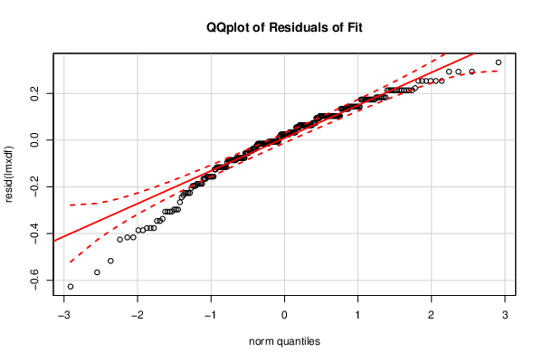
Figures (Output of Computation) | ||||||||||||||||||||||||||||||||||||||||||||||||||||||||||||||||||||||||||||||||||||||||||||||||||||||||||||||||||||||||||||||||||||||||||||||||||||||||||||||||||||||||||||||||||||||||||||
Input Parameters & R Code | ||||||||||||||||||||||||||||||||||||||||||||||||||||||||||||||||||||||||||||||||||||||||||||||||||||||||||||||||||||||||||||||||||||||||||||||||||||||||||||||||||||||||||||||||||||||||||||
| Parameters (Session): | ||||||||||||||||||||||||||||||||||||||||||||||||||||||||||||||||||||||||||||||||||||||||||||||||||||||||||||||||||||||||||||||||||||||||||||||||||||||||||||||||||||||||||||||||||||||||||||
| par1 = 1 ; par2 = 2 ; par3 = TRUE ; | ||||||||||||||||||||||||||||||||||||||||||||||||||||||||||||||||||||||||||||||||||||||||||||||||||||||||||||||||||||||||||||||||||||||||||||||||||||||||||||||||||||||||||||||||||||||||||||
| Parameters (R input): | ||||||||||||||||||||||||||||||||||||||||||||||||||||||||||||||||||||||||||||||||||||||||||||||||||||||||||||||||||||||||||||||||||||||||||||||||||||||||||||||||||||||||||||||||||||||||||||
| par1 = 1 ; par2 = 2 ; par3 = TRUE ; | ||||||||||||||||||||||||||||||||||||||||||||||||||||||||||||||||||||||||||||||||||||||||||||||||||||||||||||||||||||||||||||||||||||||||||||||||||||||||||||||||||||||||||||||||||||||||||||
| R code (references can be found in the software module): | ||||||||||||||||||||||||||||||||||||||||||||||||||||||||||||||||||||||||||||||||||||||||||||||||||||||||||||||||||||||||||||||||||||||||||||||||||||||||||||||||||||||||||||||||||||||||||||
library(boot) | ||||||||||||||||||||||||||||||||||||||||||||||||||||||||||||||||||||||||||||||||||||||||||||||||||||||||||||||||||||||||||||||||||||||||||||||||||||||||||||||||||||||||||||||||||||||||||||