Free Statistics
of Irreproducible Research!
Description of Statistical Computation | ||||||||||||||||||||||||||||||||||||||||||||||||
|---|---|---|---|---|---|---|---|---|---|---|---|---|---|---|---|---|---|---|---|---|---|---|---|---|---|---|---|---|---|---|---|---|---|---|---|---|---|---|---|---|---|---|---|---|---|---|---|---|
| Author's title | ||||||||||||||||||||||||||||||||||||||||||||||||
| Author | *The author of this computation has been verified* | |||||||||||||||||||||||||||||||||||||||||||||||
| R Software Module | rwasp_fitdistrnorm.wasp | |||||||||||||||||||||||||||||||||||||||||||||||
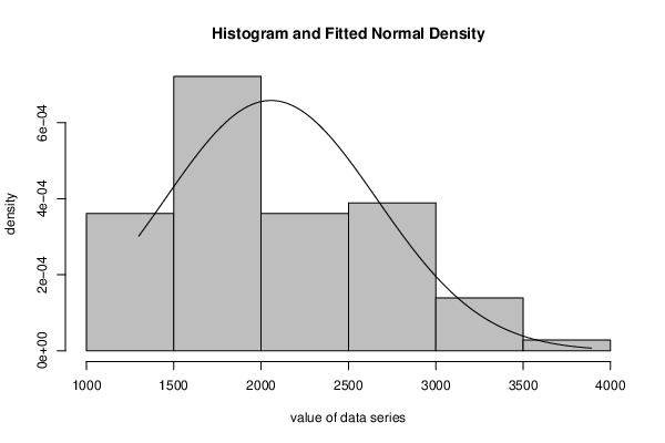
| Title produced by software | ML Fitting and QQ Plot- Normal Distribution | |||||||||||||||||||||||||||||||||||||||||||||||
| Date of computation | Thu, 31 Jan 2019 12:15:48 +0100 | |||||||||||||||||||||||||||||||||||||||||||||||
| Cite this page as follows | Statistical Computations at FreeStatistics.org, Office for Research Development and Education, URL https://freestatistics.org/blog/index.php?v=date/2019/Jan/31/t1548933369kb2x9q8gvyo2nce.htm/, Retrieved Sun, 05 May 2024 13:47:32 +0200 | |||||||||||||||||||||||||||||||||||||||||||||||
| Statistical Computations at FreeStatistics.org, Office for Research Development and Education, URL https://freestatistics.org/blog/index.php?pk=, Retrieved Sun, 05 May 2024 13:47:32 +0200 | ||||||||||||||||||||||||||||||||||||||||||||||||
| QR Codes: | ||||||||||||||||||||||||||||||||||||||||||||||||
|
| ||||||||||||||||||||||||||||||||||||||||||||||||
| Original text written by user: | ||||||||||||||||||||||||||||||||||||||||||||||||
| IsPrivate? | No (this computation is public) | |||||||||||||||||||||||||||||||||||||||||||||||
| User-defined keywords | ||||||||||||||||||||||||||||||||||||||||||||||||
| Estimated Impact | 0 | |||||||||||||||||||||||||||||||||||||||||||||||
Tree of Dependent Computations | ||||||||||||||||||||||||||||||||||||||||||||||||
Dataset | ||||||||||||||||||||||||||||||||||||||||||||||||
| Dataseries X: | ||||||||||||||||||||||||||||||||||||||||||||||||
3035 2552 2704 2554 2014 1655 1721 1524 1596 2074 2199 2512 2933 2889 2938 2497 1870 1726 1607 1545 1396 1787 2076 2837 2787 3891 3179 2011 1636 1580 1489 1300 1356 1653 2013 2823 3102 2294 2385 2444 1748 1554 1498 1361 1346 1564 1640 2293 2815 3137 2679 1969 1870 1633 1529 1366 1357 1570 1535 2491 3084 2605 2573 2143 1693 1504 1461 1354 1333 1492 1781 1915 | ||||||||||||||||||||||||||||||||||||||||||||||||
Tables (Output of Computation) | ||||||||||||||||||||||||||||||||||||||||||||||||
| ||||||||||||||||||||||||||||||||||||||||||||||||
Figures (Output of Computation) | ||||||||||||||||||||||||||||||||||||||||||||||||
Input Parameters & R Code | ||||||||||||||||||||||||||||||||||||||||||||||||
| Parameters (Session): | ||||||||||||||||||||||||||||||||||||||||||||||||
| par1 = 11111DefaultDefaultDefault1111212TRUETRUEFALSETRUETRUETRUETRUETRUE1290.360.360.360.950.95two.sided0.95two.sidedtwo.sidedgreater111111121pearsonpearsonDefault11820012Default1 2100pearson11118 ; par2 = 2222211101111110.30.30.30.30.50.365.29950200.95500.950.950.9522222221212Do not include Seasonal Dummies05121122220 ; par3 = Pearson Chi-SquaredTRUEFALSETRUE31210111111111115.355.45.355.2202050500.950.950.950.95Pearson Chi-SquaredPearson Chi-SquaredPearson Chi-SquaredTRUETRUE03No Linear Trend00Pearson Chi-Squared000.990.990.990.99 ; par4 = TRUE11011121111111115.20.050.950.95two.sidedlesstwo.sidedtwo.sided0TRUE12P1 P5 Q1 Q3 P95 P99000two.sidedtwo.sidedtwo.sidedtwo.sided ; par5 = 1212121212121212121212120.050.05pairedpairedpairedunpaired1212112unpairedpairedunpairedunpaired ; par6 = White NoiseWhite NoiseWhite Noise0330300220.00.00.00.0White Noise12White Noise00000.0 ; par7 = 0.950.950.951111111110.950.9501 ; par8 = 02202000000 ; par9 = 11111111101 ; par10 = FALSEFALSETRUE ; | ||||||||||||||||||||||||||||||||||||||||||||||||
| Parameters (R input): | ||||||||||||||||||||||||||||||||||||||||||||||||
| par1 = 8 ; par2 = 0 ; | ||||||||||||||||||||||||||||||||||||||||||||||||
| R code (references can be found in the software module): | ||||||||||||||||||||||||||||||||||||||||||||||||
library(MASS) | ||||||||||||||||||||||||||||||||||||||||||||||||