Free Statistics
of Irreproducible Research!
Description of Statistical Computation | ||||||||||||||||||||||||||||||||||||||||||||||||||||||||||||||||||||||||||||||||||||||||||||||||||||||||||||||||||||||||||||
|---|---|---|---|---|---|---|---|---|---|---|---|---|---|---|---|---|---|---|---|---|---|---|---|---|---|---|---|---|---|---|---|---|---|---|---|---|---|---|---|---|---|---|---|---|---|---|---|---|---|---|---|---|---|---|---|---|---|---|---|---|---|---|---|---|---|---|---|---|---|---|---|---|---|---|---|---|---|---|---|---|---|---|---|---|---|---|---|---|---|---|---|---|---|---|---|---|---|---|---|---|---|---|---|---|---|---|---|---|---|---|---|---|---|---|---|---|---|---|---|---|---|---|---|---|
| Author's title | ||||||||||||||||||||||||||||||||||||||||||||||||||||||||||||||||||||||||||||||||||||||||||||||||||||||||||||||||||||||||||||
| Author | *Unverified author* | |||||||||||||||||||||||||||||||||||||||||||||||||||||||||||||||||||||||||||||||||||||||||||||||||||||||||||||||||||||||||||
| R Software Module | rwasp_correlation.wasp | |||||||||||||||||||||||||||||||||||||||||||||||||||||||||||||||||||||||||||||||||||||||||||||||||||||||||||||||||||||||||||
| Title produced by software | Pearson Correlation | |||||||||||||||||||||||||||||||||||||||||||||||||||||||||||||||||||||||||||||||||||||||||||||||||||||||||||||||||||||||||||
| Date of computation | Fri, 17 May 2019 23:39:14 +0200 | |||||||||||||||||||||||||||||||||||||||||||||||||||||||||||||||||||||||||||||||||||||||||||||||||||||||||||||||||||||||||||
| Cite this page as follows | Statistical Computations at FreeStatistics.org, Office for Research Development and Education, URL https://freestatistics.org/blog/index.php?v=date/2019/May/17/t1558129323po632xlxokz45ki.htm/, Retrieved Sun, 05 May 2024 13:40:23 +0000 | |||||||||||||||||||||||||||||||||||||||||||||||||||||||||||||||||||||||||||||||||||||||||||||||||||||||||||||||||||||||||||
| Statistical Computations at FreeStatistics.org, Office for Research Development and Education, URL https://freestatistics.org/blog/index.php?pk=318817, Retrieved Sun, 05 May 2024 13:40:23 +0000 | ||||||||||||||||||||||||||||||||||||||||||||||||||||||||||||||||||||||||||||||||||||||||||||||||||||||||||||||||||||||||||||
| QR Codes: | ||||||||||||||||||||||||||||||||||||||||||||||||||||||||||||||||||||||||||||||||||||||||||||||||||||||||||||||||||||||||||||
|
| ||||||||||||||||||||||||||||||||||||||||||||||||||||||||||||||||||||||||||||||||||||||||||||||||||||||||||||||||||||||||||||
| Original text written by user: | ||||||||||||||||||||||||||||||||||||||||||||||||||||||||||||||||||||||||||||||||||||||||||||||||||||||||||||||||||||||||||||
| IsPrivate? | No (this computation is public) | |||||||||||||||||||||||||||||||||||||||||||||||||||||||||||||||||||||||||||||||||||||||||||||||||||||||||||||||||||||||||||
| User-defined keywords | ||||||||||||||||||||||||||||||||||||||||||||||||||||||||||||||||||||||||||||||||||||||||||||||||||||||||||||||||||||||||||||
| Estimated Impact | 84 | |||||||||||||||||||||||||||||||||||||||||||||||||||||||||||||||||||||||||||||||||||||||||||||||||||||||||||||||||||||||||||
Tree of Dependent Computations | ||||||||||||||||||||||||||||||||||||||||||||||||||||||||||||||||||||||||||||||||||||||||||||||||||||||||||||||||||||||||||||
| Family? (F = Feedback message, R = changed R code, M = changed R Module, P = changed Parameters, D = changed Data) | ||||||||||||||||||||||||||||||||||||||||||||||||||||||||||||||||||||||||||||||||||||||||||||||||||||||||||||||||||||||||||||
| - [Pearson Correlation] [] [2019-05-17 21:39:14] [d41d8cd98f00b204e9800998ecf8427e] [Current] | ||||||||||||||||||||||||||||||||||||||||||||||||||||||||||||||||||||||||||||||||||||||||||||||||||||||||||||||||||||||||||||
| Feedback Forum | ||||||||||||||||||||||||||||||||||||||||||||||||||||||||||||||||||||||||||||||||||||||||||||||||||||||||||||||||||||||||||||
Post a new message | ||||||||||||||||||||||||||||||||||||||||||||||||||||||||||||||||||||||||||||||||||||||||||||||||||||||||||||||||||||||||||||
Dataset | ||||||||||||||||||||||||||||||||||||||||||||||||||||||||||||||||||||||||||||||||||||||||||||||||||||||||||||||||||||||||||||
| Dataseries X: | ||||||||||||||||||||||||||||||||||||||||||||||||||||||||||||||||||||||||||||||||||||||||||||||||||||||||||||||||||||||||||||
94 94 94 94 94 94 94 153 153 153 153 153 153 153 153 153 153 293 634 1295 1295 1295 1295 1295 1295 1295 2494 2494 2494 2494 2494 2494 2494 2494 2494 2494 2494 4503 4503 4503 4503 4503 4503 4503 4503 4503 4503 475 475 475 950 950 950 1425 1425 2400 2400 2400 1650 1900 4800 729 729 729 729 729 729 729 725 725 725 725 725 725 3000 3000 3000 3000 3000 3000 3000 742 742 742 742 742 742 742 742 742 742 742 742 742 742 686 686 686 686 686 686 686 686 686 686 686 686 686 686 686 686 686 686 686 686 686 686 686 380 380 380 380 380 380 380 380 380 380 380 380 380 380 380 380 380 380 380 380 380 380 380 1450 1450 1450 1450 1450 1450 1450 1450 1450 1450 1450 1450 1450 1450 1450 1460 1460 1460 1460 1460 1460 1460 1460 1460 1460 1460 1460 1460 1460 1460 1460 1460 1460 1460 1460 1460 1460 1460 621 621 621 621 621 621 621 621 621 621 621 621 621 621 621 621 621 621 621 621 621 621 621 621 621 621 621 621 621 621 621 621 621 621 621 896 896 896 896 896 896 896 896 896 896 896 896 896 896 896 896 896 896 896 896 896 896 896 896 896 896 896 896 896 896 896 896 896 896 896 896 896 896 896 649 649 649 649 649 649 649 649 649 649 649 649 649 649 649 649 649 649 649 649 649 649 649 649 649 649 649 649 649 649 649 649 649 649 649 649 649 649 649 649 649 649 649 649 649 649 649 649 649 649 649 649 649 649 649 649 649 649 649 649 649 649 649 649 649 649 649 649 649 649 2484 2484 2484 2484 542 241 4055,5 4055,5 297 297 297 297 297 297 297 297 297 297 297 297 297 297 297 297 594 594 594 594 594 594 594 594 594 594 594 594 594 594 594 888 888 888 888 888 888 888 888 888 888 888 888 888 888 888 294 294 294 294 294 294 294 294 294 294 294 294 294 294 294 294 710 710 710 710 757 757 866 866 542 3250 3250 3250 3250 3250 3250 3250 665 665 665 665 665 665 665 665 665 665 665 665 665 665 665 665 665 665 665 665 665 665 665 665 665 665 665 665 665 665 665 665 665 665 665 665 665 665 665 665 665 665 665 665 665 665 665 665 665 665 665 665 665 665 665 665 731 731 731 731 731 731 731 731 731 731 731 1126 1126 600 600 600 600 600 600 600 600 600 600 600 600 600 600 1050 1050 1050 1050 1050 1050 1050 1050 1050 1050 1050 1050 1800 1800 1800 1800 1800 1800 1800 1800 1800 1800 1800 1050 1050 1050 1050 1050 1050 1050 1800 1800 1800 1800 1800 1800 1800 1800 1050 1050 1050 1050 1050 1050 1050 1050 1050 1050 1050 1050 1050 905 905 905 905 905 905 905 905 905 905 905 1700 1700 1700 1700 1700 1700 1700 1700 1390 1390 1390 1390 1390 1390 1390 1390 1390 1390 1390 1390 1390 1390 1034 1034 1034 1034 1034 1034 1034 1034 1034 1034 1011 1011 1011 1011 1011 1011 1011 610 610 610 610 610 610 610 610 610 610 610 610 610 610 610 610 610 610 610 610 610 610 610 610 610 610 610 610 610 610 610 610 610 610 610 610 610 610 610 610 610 610 610 610 610 610 610 610 610 610 610 610 610 610 610 610 610 610 610 610 610 610 610 610 610 610 610 610 610 610 610 610 610 610 610 610 610 610 610 610 610 610 610 610 610 610 610 610 610 610 610 610 610 610 610 610 610 875 875 875 875 875 875 875 875 875 875 875 875 875 875 875 875 875 875 875 600 600 600 600 600 600 600 600 600 600 600 1470 1470 1470 1470 1470 1470 1470 1470 1470 1128 1128 1128 1128 1128 1128 1128 1128 1128 1128 1128 1128 1128 1128 1128 1128 1128 1128 1128 1128 1128 1128 1803 1803 1803 1803 1803 1803 1803 1803 1803 1803 1803 1803 1803 1803 308 308 308 308 308 308 308 308 308 308 308 308 308 308 308 308 308 308 308 308 308 308 308 308 308 308 308 308 308 308 308 308 308 308 308 308 308 308 308 308 308 308 308 308 308 308 308 308 308 308 308 308 308 308 308 308 308 308 308 308 308 308 308 308 308 308 308 308 308 308 308 308 308 308 308 308 308 308 308 308 308 308 308 308 308 308 308 308 308 308 308 308 308 308 308 308 308 308 308 308 308 308 308 308 308 308 308 308 308 308 308 308 308 308 308 308 308 308 308 308 308 308 308 308 308 308 308 308 308 308 308 308 308 308 308 308 308 308 308 308 308 308 308 308 308 308 308 308 308 308 308 308 308 308 308 308 308 308 308 308 308 308 308 308 308 308 308 308 308 308 308 308 308 308 820 820 820 820 820 820 820 820 820 820 820 820 820 820 820 820 820 820 820 820 820 820 820 820 820 820 820 820 820 820 820 820 820 820 820 820 820 820 820 820 863 863 863 863 863 863 863 863 863 863 863 863 863 863 863 863 863 863 863 863 863 863 863 863 863 863 863 863 863 863 863 863 863 863 863 863 863 863 866 866 866 866 866 866 866 866 866 866 866 939 939 939 939 939 939 939 939 939 939 939 939 939 939 939 939 939 866 866 866 866 866 866 866 866 866 866 866 866 866 866 866 866 866 866 866 866 866 866 866 866 866 866 866 866 866 866 866 866 866 866 866 866 866 866 866 866 866 866 866 866 866 866 866 866 866 866 866 866 866 866 866 866 866 866 | ||||||||||||||||||||||||||||||||||||||||||||||||||||||||||||||||||||||||||||||||||||||||||||||||||||||||||||||||||||||||||||
| Dataseries Y: | ||||||||||||||||||||||||||||||||||||||||||||||||||||||||||||||||||||||||||||||||||||||||||||||||||||||||||||||||||||||||||||
0.06 0.06 0.06 0.06 0.06 0.06 0.06 0.1 0.1 0.1 0.1 0.1 0.1 0.1 0.1 0.1 0.1 0.17 0.43 0.59 0.59 0.59 0.59 0.59 0.59 0.59 1.20 1.20 1.20 1.20 1.20 1.20 1.20 1.20 1.20 1.20 1.20 0.87 0.87 0.87 0.87 0.87 0.87 0.87 0.87 0.87 0.87 1.71 1.71 1.71 1.64 1.64 1.64 1.99 1.99 1.47 1.47 1.47 2.43 2.97 2 533 0.61 0.61 0.61 0.61 0.61 0.61 0.61 0.69 0.69 0.69 0.69 0.69 0.69 0.75 0.75 0.75 0.75 0.75 0.75 0.75 0.29 0.29 0.29 0.29 0.29 0.29 0.29 0.7 0.7 0.7 0.7 0.7 0.7 0.7 0.36 0.36 0.36 0.36 0.36 0.36 0.36 0.36 0.36 0.36 0.36 0.7 0.7 0.7 0.7 0.7 0.7 0.7 0.7 0.7 0.7 0.7 0.7 0.12 0.12 0.12 0.12 0.12 0.12 0.12 0.12 0.12 0.12 0.12 0.12 0.12 0.12 0.12 0.12 0.12 0.12 0.12 0.12 0.12 0.12 0.12 0.27 0.27 0.27 0.27 0.27 0.27 0.27 0.27 0.27 0.27 0.27 0.27 0.27 0.27 0.27 0.32 0.32 0.32 0.32 0.32 0.32 0.32 0.32 0.32 0.32 0.32 0.32 0.32 0.32 0.32 0.32 0.32 0.32 0.32 0.32 0.32 0.32 0.32 0.18 0.18 0.18 0.18 0.18 0.18 0.18 0.18 0.18 0.18 0.18 0.18 0.18 0.18 0.18 0.18 0.18 0.18 0.18 0.18 0.18 0.18 0.18 0.18 0.18 0.18 0.18 0.18 0.18 0.18 0.18 0.18 0.18 0.18 0.96 0.88 0.88 0.88 0.88 0.88 0.88 0.88 0.88 0.88 0.88 0.88 0.88 0.88 0.88 0.88 0.88 0.88 0.88 0.88 0.88 0.88 0.88 0.88 0.88 0.88 0.88 0.88 0.88 0.88 0.88 0.88 0.88 0.88 0.88 0.88 0.88 0.88 0.88 0.88 0.8 0.8 0.8 0.8 0.8 0.8 0.8 0.8 0.8 0.8 0.8 0.8 0.8 0.8 0.8 0.8 0.8 0.8 0.8 0.8 0.8 0.8 0.8 0.8 0.8 0.8 0.8 0.8 0.8 0.8 0.8 0.8 0.8 0.8 0.8 0.8 0.8 0.8 0.8 0.8 0.8 0.8 0.8 0.8 0.8 0.8 0.8 0.8 0.8 0.8 0.8 0.8 0.8 0.8 0.8 0.8 0.8 0.8 0.8 0.8 0.8 0.8 0.8 0.8 0.8 0.8 0.8 0.8 0.8 0.8 0.96 0.96 0.96 0.96 0.88 -0.8 0.13 0.13 0.61 0.61 0.61 0.61 0.61 0.61 0.61 0.61 0.61 0.61 0.61 0.61 0.61 0.61 0.61 0.61 1.05 1.05 1.05 1.05 1.05 1.05 1.05 1.05 1.05 1.05 1.05 1.05 1.05 1.05 1.05 0.23 0.23 0.23 0.23 0.23 0.23 0.23 0.23 0.23 0.23 0.23 0.23 0.23 0.23 0.23 0.21 0.21 0.21 0.21 0.21 0.21 0.21 0.21 0.21 0.21 0.21 0.21 0.21 0.21 0.21 1.56 0.25 0.25 0.25 0.25 0.76 0.76 0.67 0.67 0.74 0.74 0.74 0.74 0.74 0.74 0.74 0.74 0.32 0.32 0.32 0.32 0.32 0.32 0.32 0.32 0.32 0.32 0.32 0.32 0.32 0.32 0.32 0.32 0.32 0.32 0.32 0.32 0.32 0.32 0.32 0.25 0.25 0.25 0.25 0.25 0.25 0.25 0.25 0.25 0.25 0.25 0.25 0.25 0.25 0.25 0.25 0.25 0.25 0.25 0.25 0.25 0.25 0.25 0.25 0.25 0.25 0.25 0.25 0.25 0.25 0.25 0.25 0.25 0.7 0.7 0.7 0.7 0.7 0.7 0.7 0.7 0.7 0.7 0.66 2.45 2.45 0.93 0.93 0.93 0.93 0.93 0.93 0.93 0.93 0.93 0.93 0.93 0.93 0.93 0.93 0.47 0.47 0.47 0.47 0.47 0.47 0.47 0.47 0.47 0.47 0.47 0.47 0.72 0.72 0.72 0.72 0.72 0.72 0.72 0.72 0.72 0.72 0.72 0.13 0.13 0.13 0.13 0.13 0.13 0.13 0.7 0.7 0.7 0.7 0.7 0.7 0.7 0.7 0.05 0.05 0.05 0.05 0.05 0.05 0.26 0.26 0.26 0.26 0.26 0.26 0.26 0.88 0.88 0.88 0.88 0.88 0.88 0.88 0.88 0.88 0.88 0.88 0.42 0.42 0.42 0.42 0.42 0.42 0.42 0.42 1.19 1.19 1.19 1.19 1.19 1.19 1.19 1.19 1.19 1.19 1.19 1.19 1.19 1.19 0.28 0.28 0.28 0.28 0.28 0.28 0.28 0.28 0.28 0.28 0.25 0.25 0.25 0.25 0.25 0.25 0.25 0.5 0.5 0.5 0.5 0.5 0.5 0.5 0.5 0.5 0.5 0.5 0.5 0.5 0.5 0.5 0.5 0.5 0.5 0.5 0.5 0.5 0.5 0.5 0.5 0.5 0.5 0.5 0.5 0.5 0.5 0.5 0.5 0.5 0.5 0.5 0.5 0.5 0.5 0.5 0.5 0.5 0.5 0.5 0.5 0.5 0.5 0.5 0.5 0.5 0.5 0.5 0.5 0.5 0.5 0.5 0.5 0.5 0.5 0.5 0.5 0.5 0.5 0.5 0.5 0.5 0.5 0.5 0.5 0.5 0.5 0.5 0.5 0.5 0.5 0.5 0.5 0.5 0.5 0.5 0.5 0.5 0.5 0.5 0.5 0.5 0.5 0.5 0.5 0.5 0.5 0.5 0.5 0.5 0.5 0.5 0.5 0.5 0.58 0.58 0.58 0.58 0.58 0.58 0.58 0.58 0.58 0.58 0.39 0.39 0.39 0.39 0.39 0.39 0.39 0.39 0.39 0.29 0.29 0.29 0.29 0.29 0.29 0.29 0.29 0.29 0.29 0.29 1.47 1.47 1.47 1.47 1.47 1.47 1.47 1.47 1.47 0.27 0.27 0.27 0.27 0.27 0.27 0.27 0.27 0.27 0.27 0.27 0.27 0.27 0.27 0.27 0.27 0.27 0.27 0.27 0.27 0.27 0.27 0.48 0.48 0.48 0.48 0.48 0.48 0.48 0.61 0.61 0.61 0.61 0.61 0.61 0.61 0.13 0.13 0.13 0.13 0.13 0.13 0.13 0.13 0.13 0.13 0.13 0.13 0.13 0.13 0.13 0.13 0.13 0.13 0.13 0.13 0.13 0.13 0.13 0.13 0.13 0.13 0.13 0.13 0.13 0.13 0.13 0.13 0.13 0.13 0.13 0.13 0.13 0.13 0.13 0.13 0.13 0.13 0.13 0.13 0.13 0.13 0.13 0.13 0.13 0.13 0.13 0.13 0.13 0.13 0.13 0.13 0.13 0.13 0.13 0.13 0.13 0.13 0.13 0.13 0.13 0.13 0.13 0.13 0.13 0.13 0.13 0.13 0.13 0.13 0.13 0.13 0.13 0.13 0.13 0.13 0.13 0.13 0.13 0.13 0.13 0.13 0.13 0.13 0.13 0.13 0.13 0.13 0.13 0.13 0.13 0.13 0.13 0.13 0.13 0.13 0.13 0.13 0.13 0.13 0.13 0.13 0.13 0.13 0.13 0.13 0.13 0.13 0.13 0.13 0.13 0.13 0.13 0.13 0.13 0.13 0.13 0.13 0.13 0.13 0.13 0.13 0.13 0.13 0.13 0.13 0.13 0.13 0.13 0.13 0.13 0.13 0.13 0.13 0.13 0.13 0.13 0.13 0.13 0.13 0.13 0.13 0.13 0.13 0.13 0.13 0.13 0.13 0.13 0.13 0.13 0.13 0.13 0.13 0.13 0.13 0.13 0.13 0.13 0.13 0.13 0.13 0.13 0.13 0.13 0.13 0.13 0.13 0.13 0.13 0.16 0.16 0.16 0.16 0.16 0.16 0.16 0.16 0.16 0.16 0.16 0.16 0.16 0.16 0.16 0.16 0.16 0.16 0.16 0.16 0.16 0.16 0.16 0.16 0.16 0.16 0.16 0.16 0.16 0.16 0.16 0.16 0.16 0.16 0.16 0.16 0.16 0.16 0.16 0.16 0.13 0.13 0.13 0.13 0.13 0.13 0.13 0.13 0.13 0.13 0.13 0.13 0.13 0.13 0.13 0.13 0.13 0.13 0.13 0.13 0.13 0.13 0.13 0.13 0.13 0.13 0.13 0.13 0.13 0.13 0.13 0.13 0.13 0.13 0.13 0.13 0.13 0.13 0.02 0.02 0.02 0.02 0.02 0.02 0.02 0.02 0.02 0.02 0.02 0.04 0.04 0.04 0.04 0.04 0.04 0.04 0.04 0.04 0.04 0.04 0.04 0.04 0.04 0.04 0.04 0.04 0.06 0.06 0.06 0.06 0.06 0.06 0.06 0.06 0.06 0.06 0.06 0.06 0.19 0.19 0.19 0.19 0.19 0.19 0.19 0.19 0.19 0.19 0.19 0.19 0.19 0.19 0.19 0.19 0.19 0.19 0.19 0.19 0.19 0.19 0.36 0.36 0.36 0.36 0.36 0.36 0.36 0.36 0.36 0.36 0.36 0.36 0.36 0.36 0.36 0.36 0.36 0.36 0.36 0.36 0.36 0.36 0.36 0.36 | ||||||||||||||||||||||||||||||||||||||||||||||||||||||||||||||||||||||||||||||||||||||||||||||||||||||||||||||||||||||||||||
Tables (Output of Computation) | ||||||||||||||||||||||||||||||||||||||||||||||||||||||||||||||||||||||||||||||||||||||||||||||||||||||||||||||||||||||||||||
| ||||||||||||||||||||||||||||||||||||||||||||||||||||||||||||||||||||||||||||||||||||||||||||||||||||||||||||||||||||||||||||
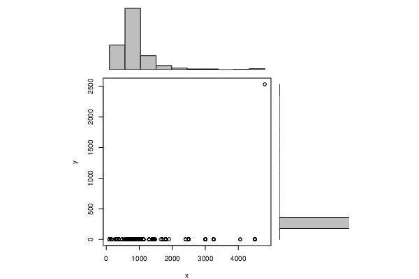
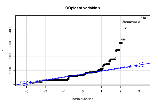
Figures (Output of Computation) | ||||||||||||||||||||||||||||||||||||||||||||||||||||||||||||||||||||||||||||||||||||||||||||||||||||||||||||||||||||||||||||
Input Parameters & R Code | ||||||||||||||||||||||||||||||||||||||||||||||||||||||||||||||||||||||||||||||||||||||||||||||||||||||||||||||||||||||||||||
| Parameters (Session): | ||||||||||||||||||||||||||||||||||||||||||||||||||||||||||||||||||||||||||||||||||||||||||||||||||||||||||||||||||||||||||||
| Parameters (R input): | ||||||||||||||||||||||||||||||||||||||||||||||||||||||||||||||||||||||||||||||||||||||||||||||||||||||||||||||||||||||||||||
| R code (references can be found in the software module): | ||||||||||||||||||||||||||||||||||||||||||||||||||||||||||||||||||||||||||||||||||||||||||||||||||||||||||||||||||||||||||||
library(psychometric) | ||||||||||||||||||||||||||||||||||||||||||||||||||||||||||||||||||||||||||||||||||||||||||||||||||||||||||||||||||||||||||||