Free Statistics
of Irreproducible Research!
Description of Statistical Computation | |||||||||||||||||||||||||||||||||||||||||||||||||||||||||||||||||||||||||||||||||
|---|---|---|---|---|---|---|---|---|---|---|---|---|---|---|---|---|---|---|---|---|---|---|---|---|---|---|---|---|---|---|---|---|---|---|---|---|---|---|---|---|---|---|---|---|---|---|---|---|---|---|---|---|---|---|---|---|---|---|---|---|---|---|---|---|---|---|---|---|---|---|---|---|---|---|---|---|---|---|---|---|---|
| Author's title | |||||||||||||||||||||||||||||||||||||||||||||||||||||||||||||||||||||||||||||||||
| Author | *Unverified author* | ||||||||||||||||||||||||||||||||||||||||||||||||||||||||||||||||||||||||||||||||
| R Software Module | rwasp_bootstrapplot.wasp | ||||||||||||||||||||||||||||||||||||||||||||||||||||||||||||||||||||||||||||||||
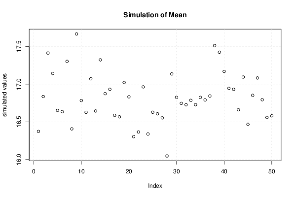
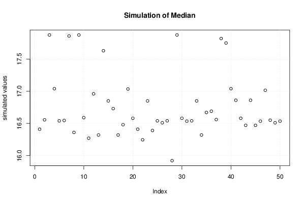
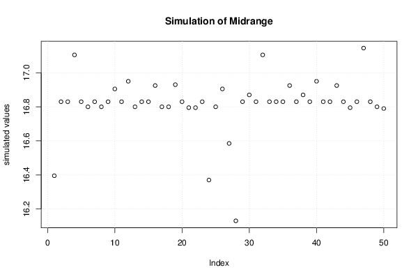
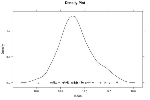
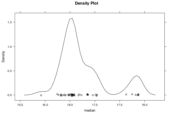
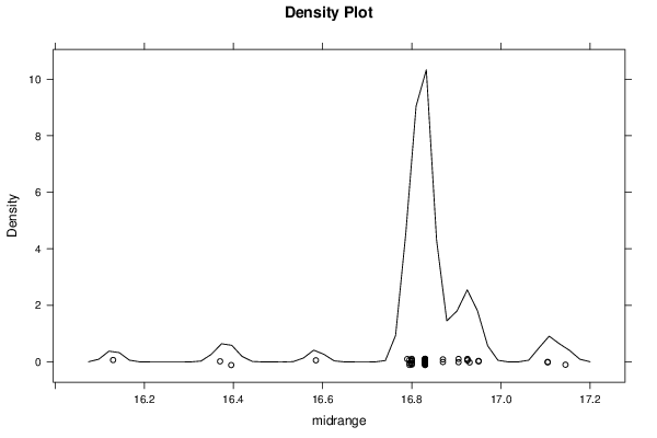
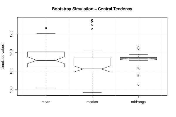
| Title produced by software | Blocked Bootstrap Plot - Central Tendency | ||||||||||||||||||||||||||||||||||||||||||||||||||||||||||||||||||||||||||||||||
| Date of computation | Fri, 24 May 2013 04:02:52 -0400 | ||||||||||||||||||||||||||||||||||||||||||||||||||||||||||||||||||||||||||||||||
| Cite this page as follows | Statistical Computations at FreeStatistics.org, Office for Research Development and Education, URL https://freestatistics.org/blog/index.php?v=date/2013/May/24/t1369382637upjuxtsks26uwl7.htm/, Retrieved Wed, 01 May 2024 05:43:19 +0000 | ||||||||||||||||||||||||||||||||||||||||||||||||||||||||||||||||||||||||||||||||
| Statistical Computations at FreeStatistics.org, Office for Research Development and Education, URL https://freestatistics.org/blog/index.php?pk=210398, Retrieved Wed, 01 May 2024 05:43:19 +0000 | |||||||||||||||||||||||||||||||||||||||||||||||||||||||||||||||||||||||||||||||||
| QR Codes: | |||||||||||||||||||||||||||||||||||||||||||||||||||||||||||||||||||||||||||||||||
|
| |||||||||||||||||||||||||||||||||||||||||||||||||||||||||||||||||||||||||||||||||
| Original text written by user: | |||||||||||||||||||||||||||||||||||||||||||||||||||||||||||||||||||||||||||||||||
| IsPrivate? | No (this computation is public) | ||||||||||||||||||||||||||||||||||||||||||||||||||||||||||||||||||||||||||||||||
| User-defined keywords | |||||||||||||||||||||||||||||||||||||||||||||||||||||||||||||||||||||||||||||||||
| Estimated Impact | 112 | ||||||||||||||||||||||||||||||||||||||||||||||||||||||||||||||||||||||||||||||||
Tree of Dependent Computations | |||||||||||||||||||||||||||||||||||||||||||||||||||||||||||||||||||||||||||||||||
| Family? (F = Feedback message, R = changed R code, M = changed R Module, P = changed Parameters, D = changed Data) | |||||||||||||||||||||||||||||||||||||||||||||||||||||||||||||||||||||||||||||||||
| - [Blocked Bootstrap Plot - Central Tendency] [] [2013-05-24 07:26:47] [709b7720e5f7ef30901a7a8e706288f1] - R P [Blocked Bootstrap Plot - Central Tendency] [] [2013-05-24 07:50:54] [709b7720e5f7ef30901a7a8e706288f1] - P [Blocked Bootstrap Plot - Central Tendency] [] [2013-05-24 07:53:39] [709b7720e5f7ef30901a7a8e706288f1] - R PD [Blocked Bootstrap Plot - Central Tendency] [Oef7 eigen reeks ] [2013-05-24 08:02:52] [09b6c15525a7e41be57b956512900af9] [Current] - R PD [Blocked Bootstrap Plot - Central Tendency] [] [2013-05-24 08:10:01] [709b7720e5f7ef30901a7a8e706288f1] - RMPD [Variability] [Oef 8 oef 1] [2013-05-24 09:55:27] [709b7720e5f7ef30901a7a8e706288f1] - RMPD [Standard Deviation Plot] [oef8 oef2] [2013-05-24 11:21:08] [709b7720e5f7ef30901a7a8e706288f1] - RMPD [Standard Deviation-Mean Plot] [oef 8 oef 2 B] [2013-05-24 12:15:08] [709b7720e5f7ef30901a7a8e706288f1] - RMPD [Variability] [oef 8 eigen reeks...] [2013-05-24 13:43:17] [709b7720e5f7ef30901a7a8e706288f1] - RMP [Standard Deviation Plot] [oef 8 eigen reeks 1B] [2013-05-24 14:42:40] [709b7720e5f7ef30901a7a8e706288f1] - RMP [Standard Deviation-Mean Plot] [oef 8 eigen reeks 1c] [2013-05-24 15:02:19] [709b7720e5f7ef30901a7a8e706288f1] - RMPD [Classical Decomposition] [oef 9 oef 1] [2013-05-24 15:07:28] [709b7720e5f7ef30901a7a8e706288f1] - RMPD [Classical Decomposition] [oef 9 oef 1] [2013-05-24 15:13:55] [709b7720e5f7ef30901a7a8e706288f1] - RMPD [Classical Decomposition] [oef 9 oef 2 eigen...] [2013-05-24 15:28:00] [709b7720e5f7ef30901a7a8e706288f1] | |||||||||||||||||||||||||||||||||||||||||||||||||||||||||||||||||||||||||||||||||
| Feedback Forum | |||||||||||||||||||||||||||||||||||||||||||||||||||||||||||||||||||||||||||||||||
Post a new message | |||||||||||||||||||||||||||||||||||||||||||||||||||||||||||||||||||||||||||||||||
Dataset | |||||||||||||||||||||||||||||||||||||||||||||||||||||||||||||||||||||||||||||||||
| Dataseries X: | |||||||||||||||||||||||||||||||||||||||||||||||||||||||||||||||||||||||||||||||||
15,58 15,66 15,73 15,74 15,77 15,78 15,8 15,81 15,82 15,88 15,85 15,89 15,92 16,02 16,1 16,13 16,21 16,25 16,27 16,21 16,21 16,24 16,32 16,32 16,36 16,48 16,54 16,58 16,56 16,55 16,58 16,53 16,6 16,46 16,48 16,48 16,49 16,54 16,67 16,72 16,79 16,86 16,84 16,86 16,96 17,01 17,02 17,04 17,04 17,39 17,54 17,57 17,58 17,56 17,63 17,67 17,71 17,75 17,82 17,86 17,89 17,96 18 18,08 18 18,02 18,01 18,02 17,95 17,96 18 18,01 | |||||||||||||||||||||||||||||||||||||||||||||||||||||||||||||||||||||||||||||||||
Tables (Output of Computation) | |||||||||||||||||||||||||||||||||||||||||||||||||||||||||||||||||||||||||||||||||
| |||||||||||||||||||||||||||||||||||||||||||||||||||||||||||||||||||||||||||||||||
Figures (Output of Computation) | |||||||||||||||||||||||||||||||||||||||||||||||||||||||||||||||||||||||||||||||||
Input Parameters & R Code | |||||||||||||||||||||||||||||||||||||||||||||||||||||||||||||||||||||||||||||||||
| Parameters (Session): | |||||||||||||||||||||||||||||||||||||||||||||||||||||||||||||||||||||||||||||||||
| par1 = 50 ; par2 = 12 ; | |||||||||||||||||||||||||||||||||||||||||||||||||||||||||||||||||||||||||||||||||
| Parameters (R input): | |||||||||||||||||||||||||||||||||||||||||||||||||||||||||||||||||||||||||||||||||
| par1 = 50 ; par2 = 12 ; | |||||||||||||||||||||||||||||||||||||||||||||||||||||||||||||||||||||||||||||||||
| R code (references can be found in the software module): | |||||||||||||||||||||||||||||||||||||||||||||||||||||||||||||||||||||||||||||||||
par1 <- as.numeric(par1) | |||||||||||||||||||||||||||||||||||||||||||||||||||||||||||||||||||||||||||||||||