Free Statistics
of Irreproducible Research!
Description of Statistical Computation | |||||||||||||||||||||||||||||||||||||||||||||
|---|---|---|---|---|---|---|---|---|---|---|---|---|---|---|---|---|---|---|---|---|---|---|---|---|---|---|---|---|---|---|---|---|---|---|---|---|---|---|---|---|---|---|---|---|---|
| Author's title | |||||||||||||||||||||||||||||||||||||||||||||
| Author | *The author of this computation has been verified* | ||||||||||||||||||||||||||||||||||||||||||||
| R Software Module | rwasp_boxcoxlin.wasp | ||||||||||||||||||||||||||||||||||||||||||||
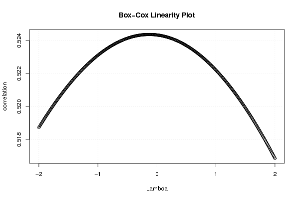
| Title produced by software | Box-Cox Linearity Plot | ||||||||||||||||||||||||||||||||||||||||||||
| Date of computation | Sun, 06 Dec 2009 08:47:52 -0700 | ||||||||||||||||||||||||||||||||||||||||||||
| Cite this page as follows | Statistical Computations at FreeStatistics.org, Office for Research Development and Education, URL https://freestatistics.org/blog/index.php?v=date/2009/Dec/06/t12601145239lsoag1x8s8zwz4.htm/, Retrieved Tue, 26 May 2026 08:17:39 +0000 | ||||||||||||||||||||||||||||||||||||||||||||
| Statistical Computations at FreeStatistics.org, Office for Research Development and Education, URL https://freestatistics.org/blog/index.php?pk=64437, Retrieved Tue, 26 May 2026 08:17:39 +0000 | |||||||||||||||||||||||||||||||||||||||||||||
| QR Codes: | |||||||||||||||||||||||||||||||||||||||||||||
|
| |||||||||||||||||||||||||||||||||||||||||||||
| Original text written by user: | |||||||||||||||||||||||||||||||||||||||||||||
| IsPrivate? | No (this computation is public) | ||||||||||||||||||||||||||||||||||||||||||||
| User-defined keywords | JSSHWPAP17 | ||||||||||||||||||||||||||||||||||||||||||||
| Estimated Impact | 503 | ||||||||||||||||||||||||||||||||||||||||||||
Tree of Dependent Computations | |||||||||||||||||||||||||||||||||||||||||||||
| Family? (F = Feedback message, R = changed R code, M = changed R Module, P = changed Parameters, D = changed Data) | |||||||||||||||||||||||||||||||||||||||||||||
| - [Notched Boxplots] [3/11/2009] [2009-11-02 21:10:41] [b98453cac15ba1066b407e146608df68] - RMPD [Univariate Explorative Data Analysis] [Tijdreeks 4] [2009-11-03 12:07:52] [214e6e00abbde49700521a7ef1d30da2] - RMPD [Kendall tau Correlation Matrix] [Kendal Tau Correl...] [2009-12-05 14:42:32] [214e6e00abbde49700521a7ef1d30da2] - RM D [Box-Cox Linearity Plot] [Box Cox Lineairit...] [2009-12-06 15:47:52] [c8fd62404619100d8e91184019148412] [Current] - RMPD [Bivariate Kernel Density Estimation] [Bivariate Kernal ...] [2009-12-10 16:40:47] [214e6e00abbde49700521a7ef1d30da2] | |||||||||||||||||||||||||||||||||||||||||||||
| Feedback Forum | |||||||||||||||||||||||||||||||||||||||||||||
Post a new message | |||||||||||||||||||||||||||||||||||||||||||||
Dataset | |||||||||||||||||||||||||||||||||||||||||||||
| Dataseries X: | |||||||||||||||||||||||||||||||||||||||||||||
369 380 474 413 537 439 355 473 435 478 450 365 315 340 326 483 406 409 423 404 551 467 332 442 305 368 411 318 398 586 367 383 533 527 418 576 359 342 456 406 374 568 335 458 456 386 457 396 366 499 354 365 594 456 366 398 468 609 418 352 | |||||||||||||||||||||||||||||||||||||||||||||
| Dataseries Y: | |||||||||||||||||||||||||||||||||||||||||||||
445 301 350 305 450 360 287 417 361 478 302 294 300 364 356 340 377 507 321 354 549 444 400 401 259 288 346 287 381 474 329 423 407 412 566 372 290 354 370 377 467 409 310 434 339 385 469 313 373 310 320 340 489 419 460 324 352 473 340 282 | |||||||||||||||||||||||||||||||||||||||||||||
Tables (Output of Computation) | |||||||||||||||||||||||||||||||||||||||||||||
| |||||||||||||||||||||||||||||||||||||||||||||
Figures (Output of Computation) | |||||||||||||||||||||||||||||||||||||||||||||
Input Parameters & R Code | |||||||||||||||||||||||||||||||||||||||||||||
| Parameters (Session): | |||||||||||||||||||||||||||||||||||||||||||||
| Parameters (R input): | |||||||||||||||||||||||||||||||||||||||||||||
| R code (references can be found in the software module): | |||||||||||||||||||||||||||||||||||||||||||||
n <- length(x) | |||||||||||||||||||||||||||||||||||||||||||||