Free Statistics
of Irreproducible Research!
Description of Statistical Computation | |||||||||||||||||||||||||||||||||||||||||||||||||||||
|---|---|---|---|---|---|---|---|---|---|---|---|---|---|---|---|---|---|---|---|---|---|---|---|---|---|---|---|---|---|---|---|---|---|---|---|---|---|---|---|---|---|---|---|---|---|---|---|---|---|---|---|---|---|
| Author's title | |||||||||||||||||||||||||||||||||||||||||||||||||||||
| Author | *The author of this computation has been verified* | ||||||||||||||||||||||||||||||||||||||||||||||||||||
| R Software Module | rwasp_edauni.wasp | ||||||||||||||||||||||||||||||||||||||||||||||||||||
| Title produced by software | Univariate Explorative Data Analysis | ||||||||||||||||||||||||||||||||||||||||||||||||||||
| Date of computation | Tue, 03 Nov 2009 05:07:52 -0700 | ||||||||||||||||||||||||||||||||||||||||||||||||||||
| Cite this page as follows | Statistical Computations at FreeStatistics.org, Office for Research Development and Education, URL https://freestatistics.org/blog/index.php?v=date/2009/Nov/03/t1257250117z2lmq3qrbzwj0nz.htm/, Retrieved Sun, 07 Dec 2025 10:38:21 +0000 | ||||||||||||||||||||||||||||||||||||||||||||||||||||
| Statistical Computations at FreeStatistics.org, Office for Research Development and Education, URL https://freestatistics.org/blog/index.php?pk=53125, Retrieved Sun, 07 Dec 2025 10:38:21 +0000 | |||||||||||||||||||||||||||||||||||||||||||||||||||||
| QR Codes: | |||||||||||||||||||||||||||||||||||||||||||||||||||||
|
| |||||||||||||||||||||||||||||||||||||||||||||||||||||
| Original text written by user: | |||||||||||||||||||||||||||||||||||||||||||||||||||||
| IsPrivate? | No (this computation is public) | ||||||||||||||||||||||||||||||||||||||||||||||||||||
| User-defined keywords | JSSHWWS6 | ||||||||||||||||||||||||||||||||||||||||||||||||||||
| Estimated Impact | 428 | ||||||||||||||||||||||||||||||||||||||||||||||||||||
Tree of Dependent Computations | |||||||||||||||||||||||||||||||||||||||||||||||||||||
| Family? (F = Feedback message, R = changed R code, M = changed R Module, P = changed Parameters, D = changed Data) | |||||||||||||||||||||||||||||||||||||||||||||||||||||
| - [Notched Boxplots] [3/11/2009] [2009-11-02 21:10:41] [b98453cac15ba1066b407e146608df68] - RMPD [Univariate Explorative Data Analysis] [Tijdreeks 4] [2009-11-03 12:07:52] [c8fd62404619100d8e91184019148412] [Current] - D [Univariate Explorative Data Analysis] [Multivariate Tijd...] [2009-12-05 14:27:17] [214e6e00abbde49700521a7ef1d30da2] - D [Univariate Explorative Data Analysis] [Multivariate Tijd...] [2009-12-05 14:29:00] [214e6e00abbde49700521a7ef1d30da2] - D [Univariate Explorative Data Analysis] [Multivariate Tijd...] [2009-12-05 14:30:27] [214e6e00abbde49700521a7ef1d30da2] - D [Univariate Explorative Data Analysis] [Multivariate Tijd...] [2009-12-05 14:31:47] [214e6e00abbde49700521a7ef1d30da2] - RMPD [Back to Back Histogram] [Back To Back Hist...] [2009-12-05 14:36:09] [214e6e00abbde49700521a7ef1d30da2] - RMPD [Kendall tau Correlation Matrix] [Kendal Tau Correl...] [2009-12-05 14:42:32] [214e6e00abbde49700521a7ef1d30da2] - RM D [Box-Cox Linearity Plot] [Box Cox Lineairit...] [2009-12-06 15:47:52] [214e6e00abbde49700521a7ef1d30da2] - RMPD [Bivariate Kernel Density Estimation] [Bivariate Kernal ...] [2009-12-10 16:40:47] [214e6e00abbde49700521a7ef1d30da2] | |||||||||||||||||||||||||||||||||||||||||||||||||||||
| Feedback Forum | |||||||||||||||||||||||||||||||||||||||||||||||||||||
Post a new message | |||||||||||||||||||||||||||||||||||||||||||||||||||||
Dataset | |||||||||||||||||||||||||||||||||||||||||||||||||||||
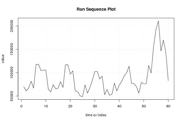
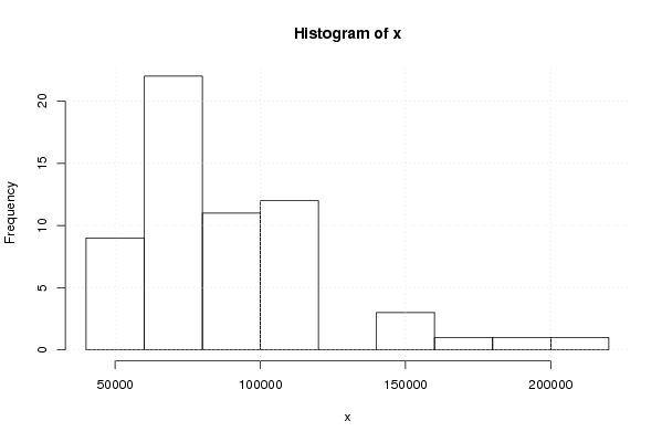
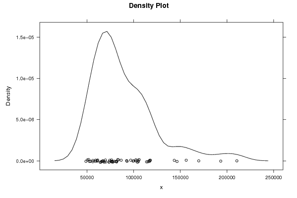
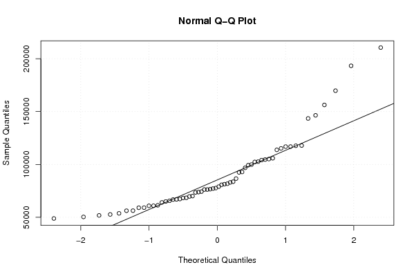
| Dataseries X: | |||||||||||||||||||||||||||||||||||||||||||||||||||||
69 698 60 886 67 267 81 723 66 938 117 673 117 873 104 619 105 074 105 856 64 918 59 006 74 269 65 562 66 752 80 732 68 229 116 882 116 855 96 773 104 083 61 344 59 094 50 330 48 842 73 817 56 173 68 407 83 658 102 355 102 600 86 598 92 442 52 663 64 042 51 768 53 708 77 648 60 830 73 504 81 314 92 861 99 861 113 777 77 159 76 573 70 059 56 245 78 970 76 239 76 244 115 187 99 296 156 275 193 294 210 544 146 442 169 727 143 482 82 977 | |||||||||||||||||||||||||||||||||||||||||||||||||||||
Tables (Output of Computation) | |||||||||||||||||||||||||||||||||||||||||||||||||||||
| |||||||||||||||||||||||||||||||||||||||||||||||||||||
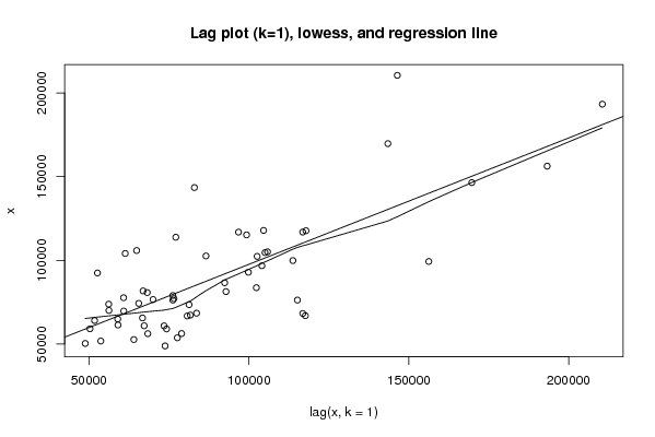
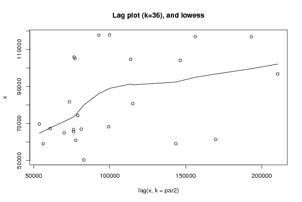
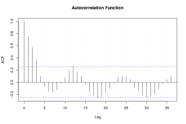
Figures (Output of Computation) | |||||||||||||||||||||||||||||||||||||||||||||||||||||
Input Parameters & R Code | |||||||||||||||||||||||||||||||||||||||||||||||||||||
| Parameters (Session): | |||||||||||||||||||||||||||||||||||||||||||||||||||||
| par1 = 0 ; par2 = 36 ; | |||||||||||||||||||||||||||||||||||||||||||||||||||||
| Parameters (R input): | |||||||||||||||||||||||||||||||||||||||||||||||||||||
| par1 = 0 ; par2 = 36 ; | |||||||||||||||||||||||||||||||||||||||||||||||||||||
| R code (references can be found in the software module): | |||||||||||||||||||||||||||||||||||||||||||||||||||||
par1 <- as.numeric(par1) | |||||||||||||||||||||||||||||||||||||||||||||||||||||