Free Statistics
of Irreproducible Research!
Description of Statistical Computation | |||||||||||||||||||||
|---|---|---|---|---|---|---|---|---|---|---|---|---|---|---|---|---|---|---|---|---|---|
| Author's title | |||||||||||||||||||||
| Author | *The author of this computation has been verified* | ||||||||||||||||||||
| R Software Module | rwasp_meanplot.wasp | ||||||||||||||||||||
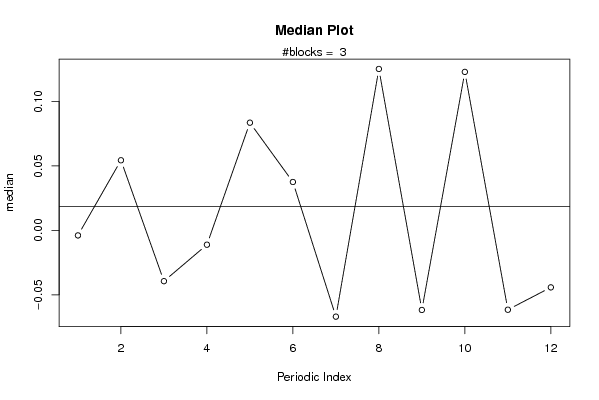
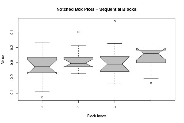
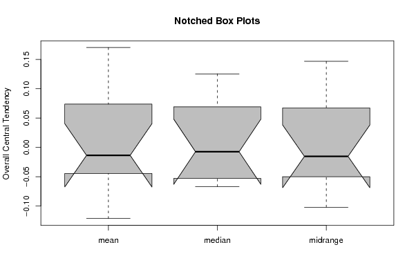
| Title produced by software | Mean Plot | ||||||||||||||||||||
| Date of computation | Mon, 07 Dec 2009 13:35:48 -0700 | ||||||||||||||||||||
| Cite this page as follows | Statistical Computations at FreeStatistics.org, Office for Research Development and Education, URL https://freestatistics.org/blog/index.php?v=date/2009/Dec/07/t12602181910hvv87t2qgsdpaq.htm/, Retrieved Sat, 27 Apr 2024 09:16:38 +0000 | ||||||||||||||||||||
| Statistical Computations at FreeStatistics.org, Office for Research Development and Education, URL https://freestatistics.org/blog/index.php?pk=64632, Retrieved Sat, 27 Apr 2024 09:16:38 +0000 | |||||||||||||||||||||
| QR Codes: | |||||||||||||||||||||
|
| |||||||||||||||||||||
| Original text written by user: | |||||||||||||||||||||
| IsPrivate? | No (this computation is public) | ||||||||||||||||||||
| User-defined keywords | |||||||||||||||||||||
| Estimated Impact | 126 | ||||||||||||||||||||
Tree of Dependent Computations | |||||||||||||||||||||
| Family? (F = Feedback message, R = changed R code, M = changed R Module, P = changed Parameters, D = changed Data) | |||||||||||||||||||||
| - [Univariate Data Series] [data set] [2008-12-01 19:54:57] [b98453cac15ba1066b407e146608df68] - RMP [ARIMA Backward Selection] [] [2009-11-27 14:53:14] [b98453cac15ba1066b407e146608df68] - PD [ARIMA Backward Selection] [] [2009-12-03 18:46:09] [90f6d58d515a4caed6fb4b8be4e11eaa] - RMPD [Mean Plot] [blog 3] [2009-12-07 20:35:48] [37de18e38c1490dd77c2b362ed87f3bb] [Current] - PD [Mean Plot] [blog 11] [2009-12-07 22:06:22] [42ad1186d39724f834063794eac7cea3] - D [Mean Plot] [blog 12] [2009-12-07 23:18:08] [42ad1186d39724f834063794eac7cea3] | |||||||||||||||||||||
| Feedback Forum | |||||||||||||||||||||
Post a new message | |||||||||||||||||||||
Dataset | |||||||||||||||||||||
| Dataseries X: | |||||||||||||||||||||
0.0268364801934054 0.268974804631799 -0.142698040626084 -0.0649895177038167 0.0877955643403605 0.0567131851744123 -0.0893170785872131 0.134075000403698 -0.378633585964905 -0.108898850310898 -0.453629669499431 -0.0442437022248864 0.062510077595423 -0.143468461277700 -0.0305889206088328 -0.0552847126011986 0.0794528506838844 0.0184331732234474 -0.0446538010417529 0.223981726197178 -0.0523367016098643 0.0513722371200867 0.40231333199086 -0.0423978557696024 -0.236840065892825 0.252370158220452 -0.0482718775183034 0.0825611235099097 0.0442032386877798 -0.0237518571796082 -0.162166669783396 -0.0101834507930462 -0.071262984201312 0.54342252788313 0.08597878503618 -0.277484540867257 -0.034642853199093 -0.267410035974983 0.116966817660426 0.0330382584768762 0.183471417812309 0.143484341422960 0.184688541573045 0.11662330405596 0.099488776130697 0.194725033551557 -0.20923056188151 | |||||||||||||||||||||
Tables (Output of Computation) | |||||||||||||||||||||
| |||||||||||||||||||||
Figures (Output of Computation) | |||||||||||||||||||||
Input Parameters & R Code | |||||||||||||||||||||
| Parameters (Session): | |||||||||||||||||||||
| par1 = 12 ; | |||||||||||||||||||||
| Parameters (R input): | |||||||||||||||||||||
| par1 = 12 ; | |||||||||||||||||||||
| R code (references can be found in the software module): | |||||||||||||||||||||
par1 <- as.numeric(par1) | |||||||||||||||||||||