Free Statistics
of Irreproducible Research!
Description of Statistical Computation | |||||||||||||||||||||
|---|---|---|---|---|---|---|---|---|---|---|---|---|---|---|---|---|---|---|---|---|---|
| Author's title | |||||||||||||||||||||
| Author | *The author of this computation has been verified* | ||||||||||||||||||||
| R Software Module | rwasp_meanplot.wasp | ||||||||||||||||||||
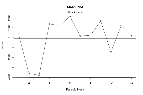
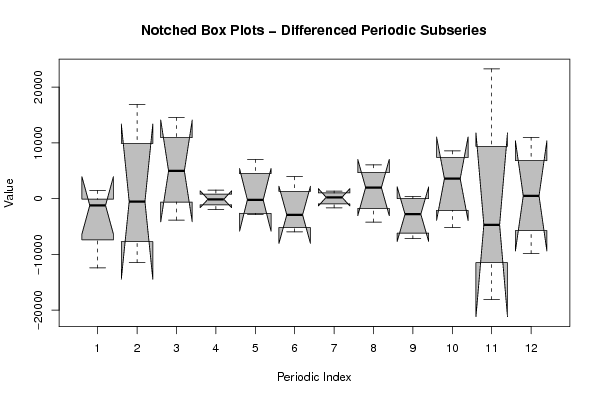
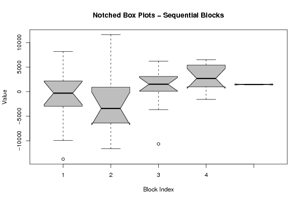
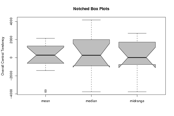
| Title produced by software | Mean Plot | ||||||||||||||||||||
| Date of computation | Mon, 07 Dec 2009 15:06:22 -0700 | ||||||||||||||||||||
| Cite this page as follows | Statistical Computations at FreeStatistics.org, Office for Research Development and Education, URL https://freestatistics.org/blog/index.php?v=date/2009/Dec/07/t1260223612xi3tkg8jas6u8s2.htm/, Retrieved Wed, 13 May 2026 06:47:10 +0000 | ||||||||||||||||||||
| Statistical Computations at FreeStatistics.org, Office for Research Development and Education, URL https://freestatistics.org/blog/index.php?pk=64651, Retrieved Wed, 13 May 2026 06:47:10 +0000 | |||||||||||||||||||||
| QR Codes: | |||||||||||||||||||||
|
| |||||||||||||||||||||
| Original text written by user: | |||||||||||||||||||||
| IsPrivate? | No (this computation is public) | ||||||||||||||||||||
| User-defined keywords | |||||||||||||||||||||
| Estimated Impact | 403 | ||||||||||||||||||||
Tree of Dependent Computations | |||||||||||||||||||||
| Family? (F = Feedback message, R = changed R code, M = changed R Module, P = changed Parameters, D = changed Data) | |||||||||||||||||||||
| - [Univariate Data Series] [data set] [2008-12-01 19:54:57] [b98453cac15ba1066b407e146608df68] - RMP [ARIMA Backward Selection] [] [2009-11-27 14:53:14] [b98453cac15ba1066b407e146608df68] - PD [ARIMA Backward Selection] [] [2009-12-03 18:46:09] [90f6d58d515a4caed6fb4b8be4e11eaa] - RMPD [Mean Plot] [blog 3] [2009-12-07 20:35:48] [42ad1186d39724f834063794eac7cea3] - PD [Mean Plot] [blog 11] [2009-12-07 22:06:22] [37de18e38c1490dd77c2b362ed87f3bb] [Current] | |||||||||||||||||||||
| Feedback Forum | |||||||||||||||||||||
Post a new message | |||||||||||||||||||||
Dataset | |||||||||||||||||||||
| Dataseries X: | |||||||||||||||||||||
-1065.28076055322 -2278.75083745204 -13750.7320730183 768.487940174182 480.329421548304 2441.84534097982 -2017.12122801278 -3677.24413007058 2376.07844077739 1991.57956111441 8177.8663887305 -9931.36901798728 1054.78346037674 -6334.48912633556 -10318.8992855633 -2985.24764365473 -4927.33781231944 2075.02534260383 -3870.63118024471 -2524.15412506803 725.810856004154 -6465.06532185037 -11625.1356478526 11621.1659938228 1767.57466477775 -10664.0704054107 6189.98081853049 2343.11555395316 3876.36005581636 1472.93269355467 118.383083333785 820.674136304355 1542.41090621852 -3650.11001150461 4906.01253028907 40.3638959194068 -1585.17421898316 -124.437694132677 2791.13055865956 5387.15230614261 5445.44402054302 2593.37824514089 6516.19939614798 6292.59289700375 2088.48664589605 2475.88763066489 3427.36476553255 -1086.08268469240 1510.63701057434 1414.23900224041 | |||||||||||||||||||||
Tables (Output of Computation) | |||||||||||||||||||||
| |||||||||||||||||||||
Figures (Output of Computation) | |||||||||||||||||||||
Input Parameters & R Code | |||||||||||||||||||||
| Parameters (Session): | |||||||||||||||||||||
| par1 = 36 ; par2 = 1 ; par3 = 1 ; par4 = 1 ; par5 = 12 ; par6 = MA ; par7 = 0.95 ; | |||||||||||||||||||||
| Parameters (R input): | |||||||||||||||||||||
| par1 = 12 ; | |||||||||||||||||||||
| R code (references can be found in the software module): | |||||||||||||||||||||
par1 <- as.numeric(par1) | |||||||||||||||||||||