Repository of Reproducible Computations

Free Statistics

of Irreproducible Research!

Author's title

Author

*The author of this computation has been verified*

R Software Module

rwasp_autocorrelation.wasp

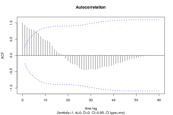
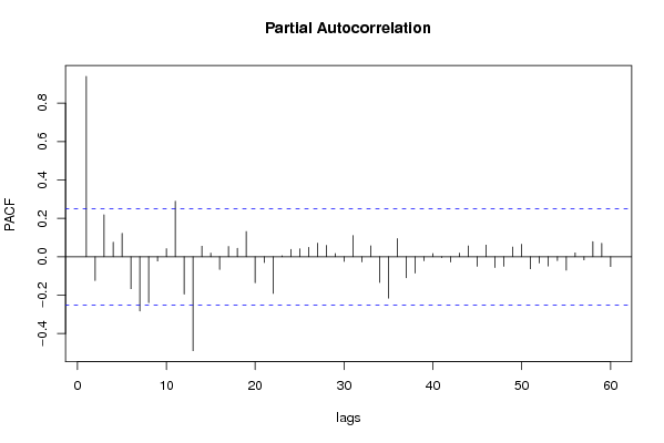
Title produced by software

(Partial) Autocorrelation Function

Date of computation

Sat, 19 Dec 2009 04:26:01 -0700

Cite this page as follows

Statistical Computations at FreeStatistics.org, Office for Research Development and Education, URL https://freestatistics.org/blog/index.php?v=date/2009/Dec/19/t1261222004enc3fhuudnjcu6y.htm/, Retrieved Mon, 29 Apr 2024 09:28:21 +0000

Statistical Computations at FreeStatistics.org, Office for Research Development and Education, URL https://freestatistics.org/blog/index.php?pk=69510, Retrieved Mon, 29 Apr 2024 09:28:21 +0000

QR Codes:

Paste this QR Code to cite your computation.

Original text written by user:

IsPrivate?

No (this computation is public)

User-defined keywords

Estimated Impact

149

Family? (F = Feedback message, R = changed R code, M = changed R Module, P = changed Parameters, D = changed Data)

-     [Univariate Explorative Data Analysis] [Run Sequence gebo...] [2008-12-12 13:32:37] [76963dc1903f0f612b6153510a3818cf]
- R  D  [Univariate Explorative Data Analysis] [Run Sequence gebo...] [2008-12-17 12:14:40] [76963dc1903f0f612b6153510a3818cf]
-         [Univariate Explorative Data Analysis] [Run Sequence Plot...] [2008-12-22 18:19:51] [1ce0d16c8f4225c977b42c8fa93bc163]
- RMP       [(Partial) Autocorrelation Function] [Identifying Integ...] [2009-11-22 12:16:10] [b98453cac15ba1066b407e146608df68]
-    D        [(Partial) Autocorrelation Function] [Autocorrelatie fu...] [2009-11-23 18:29:14] [d46757a0a8c9b00540ab7e7e0c34bfc4]
-    D          [(Partial) Autocorrelation Function] [ACF met: d=0, D=0...] [2009-12-03 22:50:11] [34d27ebe78dc2d31581e8710befe8733]
-    D            [(Partial) Autocorrelation Function] [ACF met: d=0, D=0...] [2009-12-16 22:39:45] [34d27ebe78dc2d31581e8710befe8733]
-   P                 [(Partial) Autocorrelation Function] [ACF met: d=0, D=0...] [2009-12-19 11:26:01] [371dc2189c569d90e2c1567f632c3ec0] [Current]

Feedback Forum

Post a new message

Dataseries X:

Download CSV

Histogram

Boxplots

Summary of computational transaction
Raw Input	view raw input (R code)
Raw Output	view raw output of R engine
Computing time	1 seconds
R Server	'Gwilym Jenkins' @ 72.249.127.135

\begin{tabular}{lllllllll}
\hline
Summary of computational transaction \tabularnewline
Raw Input & view raw input (R code)  \tabularnewline
Raw Output & view raw output of R engine  \tabularnewline
Computing time & 1 seconds \tabularnewline
R Server & 'Gwilym Jenkins' @ 72.249.127.135 \tabularnewline
\hline
\end{tabular}
%Source: https://freestatistics.org/blog/index.php?pk=69510&T=0

[TABLE]
[ROW][C]Summary of computational transaction[/C][/ROW]
[ROW][C]Raw Input[/C][C]view raw input (R code) [/C][/ROW]
[ROW][C]Raw Output[/C][C]view raw output of R engine [/C][/ROW]
[ROW][C]Computing time[/C][C]1 seconds[/C][/ROW]
[ROW][C]R Server[/C][C]'Gwilym Jenkins' @ 72.249.127.135[/C][/ROW]
[/TABLE]
Source: https://freestatistics.org/blog/index.php?pk=69510&T=0

Globally Unique Identifier (entire table): ba.freestatistics.org/blog/index.php?pk=69510&T=0

As an alternative you can also use a QR Code:

The GUIDs for individual cells are displayed in the table below:

Summary of computational transaction
Raw Input	view raw input (R code)
Raw Output	view raw output of R engine
Computing time	1 seconds
R Server	'Gwilym Jenkins' @ 72.249.127.135

Autocorrelation Function
Time lag k	ACF(k)	T-STAT	P-value
1	0.939502	7.3377	0
2	0.868119	6.7802	0
3	0.825505	6.4474	0
4	0.799813	6.2467	0
5	0.78541	6.1342	0
6	0.750111	5.8586	0
7	0.675882	5.2788	1e-06
8	0.583499	4.5573	1.3e-05
9	0.510936	3.9905	9e-05
10	0.465947	3.6392	0.000282
11	0.452439	3.5337	0.000394
12	0.407766	3.1848	0.001141
13	0.294251	2.2982	0.012497
14	0.19285	1.5062	0.068588
15	0.121728	0.9507	0.172748
16	0.067934	0.5306	0.298818
17	0.032387	0.2529	0.400579
18	-0.016015	-0.1251	0.450434
19	-0.08854	-0.6915	0.245932
20	-0.17316	-1.3524	0.090616
21	-0.231029	-1.8044	0.038053
22	-0.263215	-2.0558	0.022046
23	-0.272475	-2.1281	0.018689
24	-0.307303	-2.4001	0.009729
25	-0.375366	-2.9317	0.00237
26	-0.421862	-3.2948	0.000822
27	-0.44511	-3.4764	0.000471
28	-0.447572	-3.4956	0.000444
29	-0.432026	-3.3742	0.000646
30	-0.422195	-3.2974	0.000815
31	-0.425574	-3.3238	0.000753
32	-0.433714	-3.3874	0.00062
33	-0.417438	-3.2603	0.000911
34	-0.387171	-3.0239	0.001824
35	-0.357359	-2.7911	0.003502
36	-0.33891	-2.647	0.00516
37	-0.342393	-2.6742	0.0048
38	-0.335605	-2.6212	0.005524
39	-0.319224	-2.4932	0.007694
40	-0.290824	-2.2714	0.013331
41	-0.25981	-2.0292	0.023405
42	-0.233414	-1.823	0.036601
43	-0.217008	-1.6949	0.047599
44	-0.201074	-1.5704	0.060743
45	-0.173089	-1.3519	0.090705
46	-0.144965	-1.1322	0.130988
47	-0.119365	-0.9323	0.177437
48	-0.09991	-0.7803	0.219109
49	-0.091255	-0.7127	0.239366
50	-0.073712	-0.5757	0.283466
51	-0.054369	-0.4246	0.336298
52	-0.03434	-0.2682	0.394723
53	-0.020725	-0.1619	0.435972
54	-0.011636	-0.0909	0.463943
55	-0.006504	-0.0508	0.479825
56	-0.003037	-0.0237	0.490578
57	0.00455	0.0355	0.485885
58	0.003818	0.0298	0.488155
59	0.0045	0.0351	0.48604
60	0.001349	0.0105	0.495815

\begin{tabular}{lllllllll}
\hline
Autocorrelation Function \tabularnewline
Time lag k & ACF(k) & T-STAT & P-value \tabularnewline
1 & 0.939502 & 7.3377 & 0 \tabularnewline
2 & 0.868119 & 6.7802 & 0 \tabularnewline
3 & 0.825505 & 6.4474 & 0 \tabularnewline
4 & 0.799813 & 6.2467 & 0 \tabularnewline
5 & 0.78541 & 6.1342 & 0 \tabularnewline
6 & 0.750111 & 5.8586 & 0 \tabularnewline
7 & 0.675882 & 5.2788 & 1e-06 \tabularnewline
8 & 0.583499 & 4.5573 & 1.3e-05 \tabularnewline
9 & 0.510936 & 3.9905 & 9e-05 \tabularnewline
10 & 0.465947 & 3.6392 & 0.000282 \tabularnewline
11 & 0.452439 & 3.5337 & 0.000394 \tabularnewline
12 & 0.407766 & 3.1848 & 0.001141 \tabularnewline
13 & 0.294251 & 2.2982 & 0.012497 \tabularnewline
14 & 0.19285 & 1.5062 & 0.068588 \tabularnewline
15 & 0.121728 & 0.9507 & 0.172748 \tabularnewline
16 & 0.067934 & 0.5306 & 0.298818 \tabularnewline
17 & 0.032387 & 0.2529 & 0.400579 \tabularnewline
18 & -0.016015 & -0.1251 & 0.450434 \tabularnewline
19 & -0.08854 & -0.6915 & 0.245932 \tabularnewline
20 & -0.17316 & -1.3524 & 0.090616 \tabularnewline
21 & -0.231029 & -1.8044 & 0.038053 \tabularnewline
22 & -0.263215 & -2.0558 & 0.022046 \tabularnewline
23 & -0.272475 & -2.1281 & 0.018689 \tabularnewline
24 & -0.307303 & -2.4001 & 0.009729 \tabularnewline
25 & -0.375366 & -2.9317 & 0.00237 \tabularnewline
26 & -0.421862 & -3.2948 & 0.000822 \tabularnewline
27 & -0.44511 & -3.4764 & 0.000471 \tabularnewline
28 & -0.447572 & -3.4956 & 0.000444 \tabularnewline
29 & -0.432026 & -3.3742 & 0.000646 \tabularnewline
30 & -0.422195 & -3.2974 & 0.000815 \tabularnewline
31 & -0.425574 & -3.3238 & 0.000753 \tabularnewline
32 & -0.433714 & -3.3874 & 0.00062 \tabularnewline
33 & -0.417438 & -3.2603 & 0.000911 \tabularnewline
34 & -0.387171 & -3.0239 & 0.001824 \tabularnewline
35 & -0.357359 & -2.7911 & 0.003502 \tabularnewline
36 & -0.33891 & -2.647 & 0.00516 \tabularnewline
37 & -0.342393 & -2.6742 & 0.0048 \tabularnewline
38 & -0.335605 & -2.6212 & 0.005524 \tabularnewline
39 & -0.319224 & -2.4932 & 0.007694 \tabularnewline
40 & -0.290824 & -2.2714 & 0.013331 \tabularnewline
41 & -0.25981 & -2.0292 & 0.023405 \tabularnewline
42 & -0.233414 & -1.823 & 0.036601 \tabularnewline
43 & -0.217008 & -1.6949 & 0.047599 \tabularnewline
44 & -0.201074 & -1.5704 & 0.060743 \tabularnewline
45 & -0.173089 & -1.3519 & 0.090705 \tabularnewline
46 & -0.144965 & -1.1322 & 0.130988 \tabularnewline
47 & -0.119365 & -0.9323 & 0.177437 \tabularnewline
48 & -0.09991 & -0.7803 & 0.219109 \tabularnewline
49 & -0.091255 & -0.7127 & 0.239366 \tabularnewline
50 & -0.073712 & -0.5757 & 0.283466 \tabularnewline
51 & -0.054369 & -0.4246 & 0.336298 \tabularnewline
52 & -0.03434 & -0.2682 & 0.394723 \tabularnewline
53 & -0.020725 & -0.1619 & 0.435972 \tabularnewline
54 & -0.011636 & -0.0909 & 0.463943 \tabularnewline
55 & -0.006504 & -0.0508 & 0.479825 \tabularnewline
56 & -0.003037 & -0.0237 & 0.490578 \tabularnewline
57 & 0.00455 & 0.0355 & 0.485885 \tabularnewline
58 & 0.003818 & 0.0298 & 0.488155 \tabularnewline
59 & 0.0045 & 0.0351 & 0.48604 \tabularnewline
60 & 0.001349 & 0.0105 & 0.495815 \tabularnewline
\hline
\end{tabular}
%Source: https://freestatistics.org/blog/index.php?pk=69510&T=1

[TABLE]
[ROW][C]Autocorrelation Function[/C][/ROW]
[ROW][C]Time lag k[/C][C]ACF(k)[/C][C]T-STAT[/C][C]P-value[/C][/ROW]
[ROW][C]1[/C][C]0.939502[/C][C]7.3377[/C][C]0[/C][/ROW]
[ROW][C]2[/C][C]0.868119[/C][C]6.7802[/C][C]0[/C][/ROW]
[ROW][C]3[/C][C]0.825505[/C][C]6.4474[/C][C]0[/C][/ROW]
[ROW][C]4[/C][C]0.799813[/C][C]6.2467[/C][C]0[/C][/ROW]
[ROW][C]5[/C][C]0.78541[/C][C]6.1342[/C][C]0[/C][/ROW]
[ROW][C]6[/C][C]0.750111[/C][C]5.8586[/C][C]0[/C][/ROW]
[ROW][C]7[/C][C]0.675882[/C][C]5.2788[/C][C]1e-06[/C][/ROW]
[ROW][C]8[/C][C]0.583499[/C][C]4.5573[/C][C]1.3e-05[/C][/ROW]
[ROW][C]9[/C][C]0.510936[/C][C]3.9905[/C][C]9e-05[/C][/ROW]
[ROW][C]10[/C][C]0.465947[/C][C]3.6392[/C][C]0.000282[/C][/ROW]
[ROW][C]11[/C][C]0.452439[/C][C]3.5337[/C][C]0.000394[/C][/ROW]
[ROW][C]12[/C][C]0.407766[/C][C]3.1848[/C][C]0.001141[/C][/ROW]
[ROW][C]13[/C][C]0.294251[/C][C]2.2982[/C][C]0.012497[/C][/ROW]
[ROW][C]14[/C][C]0.19285[/C][C]1.5062[/C][C]0.068588[/C][/ROW]
[ROW][C]15[/C][C]0.121728[/C][C]0.9507[/C][C]0.172748[/C][/ROW]
[ROW][C]16[/C][C]0.067934[/C][C]0.5306[/C][C]0.298818[/C][/ROW]
[ROW][C]17[/C][C]0.032387[/C][C]0.2529[/C][C]0.400579[/C][/ROW]
[ROW][C]18[/C][C]-0.016015[/C][C]-0.1251[/C][C]0.450434[/C][/ROW]
[ROW][C]19[/C][C]-0.08854[/C][C]-0.6915[/C][C]0.245932[/C][/ROW]
[ROW][C]20[/C][C]-0.17316[/C][C]-1.3524[/C][C]0.090616[/C][/ROW]
[ROW][C]21[/C][C]-0.231029[/C][C]-1.8044[/C][C]0.038053[/C][/ROW]
[ROW][C]22[/C][C]-0.263215[/C][C]-2.0558[/C][C]0.022046[/C][/ROW]
[ROW][C]23[/C][C]-0.272475[/C][C]-2.1281[/C][C]0.018689[/C][/ROW]
[ROW][C]24[/C][C]-0.307303[/C][C]-2.4001[/C][C]0.009729[/C][/ROW]
[ROW][C]25[/C][C]-0.375366[/C][C]-2.9317[/C][C]0.00237[/C][/ROW]
[ROW][C]26[/C][C]-0.421862[/C][C]-3.2948[/C][C]0.000822[/C][/ROW]
[ROW][C]27[/C][C]-0.44511[/C][C]-3.4764[/C][C]0.000471[/C][/ROW]
[ROW][C]28[/C][C]-0.447572[/C][C]-3.4956[/C][C]0.000444[/C][/ROW]
[ROW][C]29[/C][C]-0.432026[/C][C]-3.3742[/C][C]0.000646[/C][/ROW]
[ROW][C]30[/C][C]-0.422195[/C][C]-3.2974[/C][C]0.000815[/C][/ROW]
[ROW][C]31[/C][C]-0.425574[/C][C]-3.3238[/C][C]0.000753[/C][/ROW]
[ROW][C]32[/C][C]-0.433714[/C][C]-3.3874[/C][C]0.00062[/C][/ROW]
[ROW][C]33[/C][C]-0.417438[/C][C]-3.2603[/C][C]0.000911[/C][/ROW]
[ROW][C]34[/C][C]-0.387171[/C][C]-3.0239[/C][C]0.001824[/C][/ROW]
[ROW][C]35[/C][C]-0.357359[/C][C]-2.7911[/C][C]0.003502[/C][/ROW]
[ROW][C]36[/C][C]-0.33891[/C][C]-2.647[/C][C]0.00516[/C][/ROW]
[ROW][C]37[/C][C]-0.342393[/C][C]-2.6742[/C][C]0.0048[/C][/ROW]
[ROW][C]38[/C][C]-0.335605[/C][C]-2.6212[/C][C]0.005524[/C][/ROW]
[ROW][C]39[/C][C]-0.319224[/C][C]-2.4932[/C][C]0.007694[/C][/ROW]
[ROW][C]40[/C][C]-0.290824[/C][C]-2.2714[/C][C]0.013331[/C][/ROW]
[ROW][C]41[/C][C]-0.25981[/C][C]-2.0292[/C][C]0.023405[/C][/ROW]
[ROW][C]42[/C][C]-0.233414[/C][C]-1.823[/C][C]0.036601[/C][/ROW]
[ROW][C]43[/C][C]-0.217008[/C][C]-1.6949[/C][C]0.047599[/C][/ROW]
[ROW][C]44[/C][C]-0.201074[/C][C]-1.5704[/C][C]0.060743[/C][/ROW]
[ROW][C]45[/C][C]-0.173089[/C][C]-1.3519[/C][C]0.090705[/C][/ROW]
[ROW][C]46[/C][C]-0.144965[/C][C]-1.1322[/C][C]0.130988[/C][/ROW]
[ROW][C]47[/C][C]-0.119365[/C][C]-0.9323[/C][C]0.177437[/C][/ROW]
[ROW][C]48[/C][C]-0.09991[/C][C]-0.7803[/C][C]0.219109[/C][/ROW]
[ROW][C]49[/C][C]-0.091255[/C][C]-0.7127[/C][C]0.239366[/C][/ROW]
[ROW][C]50[/C][C]-0.073712[/C][C]-0.5757[/C][C]0.283466[/C][/ROW]
[ROW][C]51[/C][C]-0.054369[/C][C]-0.4246[/C][C]0.336298[/C][/ROW]
[ROW][C]52[/C][C]-0.03434[/C][C]-0.2682[/C][C]0.394723[/C][/ROW]
[ROW][C]53[/C][C]-0.020725[/C][C]-0.1619[/C][C]0.435972[/C][/ROW]
[ROW][C]54[/C][C]-0.011636[/C][C]-0.0909[/C][C]0.463943[/C][/ROW]
[ROW][C]55[/C][C]-0.006504[/C][C]-0.0508[/C][C]0.479825[/C][/ROW]
[ROW][C]56[/C][C]-0.003037[/C][C]-0.0237[/C][C]0.490578[/C][/ROW]
[ROW][C]57[/C][C]0.00455[/C][C]0.0355[/C][C]0.485885[/C][/ROW]
[ROW][C]58[/C][C]0.003818[/C][C]0.0298[/C][C]0.488155[/C][/ROW]
[ROW][C]59[/C][C]0.0045[/C][C]0.0351[/C][C]0.48604[/C][/ROW]
[ROW][C]60[/C][C]0.001349[/C][C]0.0105[/C][C]0.495815[/C][/ROW]
[/TABLE]
Source: https://freestatistics.org/blog/index.php?pk=69510&T=1

Globally Unique Identifier (entire table): ba.freestatistics.org/blog/index.php?pk=69510&T=1

As an alternative you can also use a QR Code:

The GUIDs for individual cells are displayed in the table below:

Autocorrelation Function
Time lag k	ACF(k)	T-STAT	P-value
1	0.939502	7.3377	0
2	0.868119	6.7802	0
3	0.825505	6.4474	0
4	0.799813	6.2467	0
5	0.78541	6.1342	0
6	0.750111	5.8586	0
7	0.675882	5.2788	1e-06
8	0.583499	4.5573	1.3e-05
9	0.510936	3.9905	9e-05
10	0.465947	3.6392	0.000282
11	0.452439	3.5337	0.000394
12	0.407766	3.1848	0.001141
13	0.294251	2.2982	0.012497
14	0.19285	1.5062	0.068588
15	0.121728	0.9507	0.172748
16	0.067934	0.5306	0.298818
17	0.032387	0.2529	0.400579
18	-0.016015	-0.1251	0.450434
19	-0.08854	-0.6915	0.245932
20	-0.17316	-1.3524	0.090616
21	-0.231029	-1.8044	0.038053
22	-0.263215	-2.0558	0.022046
23	-0.272475	-2.1281	0.018689
24	-0.307303	-2.4001	0.009729
25	-0.375366	-2.9317	0.00237
26	-0.421862	-3.2948	0.000822
27	-0.44511	-3.4764	0.000471
28	-0.447572	-3.4956	0.000444
29	-0.432026	-3.3742	0.000646
30	-0.422195	-3.2974	0.000815
31	-0.425574	-3.3238	0.000753
32	-0.433714	-3.3874	0.00062
33	-0.417438	-3.2603	0.000911
34	-0.387171	-3.0239	0.001824
35	-0.357359	-2.7911	0.003502
36	-0.33891	-2.647	0.00516
37	-0.342393	-2.6742	0.0048
38	-0.335605	-2.6212	0.005524
39	-0.319224	-2.4932	0.007694
40	-0.290824	-2.2714	0.013331
41	-0.25981	-2.0292	0.023405
42	-0.233414	-1.823	0.036601
43	-0.217008	-1.6949	0.047599
44	-0.201074	-1.5704	0.060743
45	-0.173089	-1.3519	0.090705
46	-0.144965	-1.1322	0.130988
47	-0.119365	-0.9323	0.177437
48	-0.09991	-0.7803	0.219109
49	-0.091255	-0.7127	0.239366
50	-0.073712	-0.5757	0.283466
51	-0.054369	-0.4246	0.336298
52	-0.03434	-0.2682	0.394723
53	-0.020725	-0.1619	0.435972
54	-0.011636	-0.0909	0.463943
55	-0.006504	-0.0508	0.479825
56	-0.003037	-0.0237	0.490578
57	0.00455	0.0355	0.485885
58	0.003818	0.0298	0.488155
59	0.0045	0.0351	0.48604
60	0.001349	0.0105	0.495815

Partial Autocorrelation Function
Time lag k	PACF(k)	T-STAT	P-value
1	0.939502	7.3377	0
2	-0.123964	-0.9682	0.168387
3	0.218674	1.7079	0.04637
4	0.075996	0.5936	0.277504
5	0.1221	0.9536	0.172017
6	-0.166059	-1.297	0.099764
7	-0.282051	-2.2029	0.015695
8	-0.239013	-1.8668	0.033372
9	-0.022069	-0.1724	0.431861
10	0.042039	0.3283	0.371891
11	0.289238	2.259	0.013734
12	-0.194093	-1.5159	0.067354
13	-0.488952	-3.8188	0.000158
14	0.055418	0.4328	0.333333
15	0.019358	0.1512	0.440161
16	-0.066189	-0.517	0.30353
17	0.053541	0.4182	0.338647
18	0.04456	0.348	0.364509
19	0.131254	1.0251	0.154677
20	-0.13494	-1.0539	0.148039
21	-0.030032	-0.2346	0.40767
22	-0.190775	-1.49	0.070688
23	0.005397	0.0422	0.483258
24	0.038772	0.3028	0.381528
25	0.041155	0.3214	0.374491
26	0.048999	0.3827	0.351638
27	0.071044	0.5549	0.290505
28	0.059709	0.4663	0.321317
29	0.016845	0.1316	0.447881
30	-0.024379	-0.1904	0.424813
31	0.110942	0.8665	0.194809
32	-0.026513	-0.2071	0.41832
33	0.057254	0.4472	0.32817
34	-0.133927	-1.046	0.149843
35	-0.21504	-1.6795	0.049083
36	0.094939	0.7415	0.230618
37	-0.10924	-0.8532	0.198446
38	-0.084831	-0.6625	0.255057
39	-0.020679	-0.1615	0.436113
40	0.017175	0.1341	0.446867
41	-0.004191	-0.0327	0.486998
42	-0.026803	-0.2093	0.41744
43	0.019292	0.1507	0.440366
44	0.056798	0.4436	0.329449
45	-0.04939	-0.3857	0.350513
46	0.060776	0.4747	0.318356
47	-0.05576	-0.4355	0.332368
48	-0.049814	-0.3891	0.349293
49	0.05098	0.3982	0.345949
50	0.065178	0.5091	0.306275
51	-0.062331	-0.4868	0.314064
52	-0.032517	-0.254	0.40019
53	-0.047685	-0.3724	0.35543
54	-0.01994	-0.1557	0.438377
55	-0.069459	-0.5425	0.294728
56	0.020458	0.1598	0.43679
57	-0.016272	-0.1271	0.449644
58	0.078577	0.6137	0.270845
59	0.070146	0.5479	0.292894
60	-0.051255	-0.4003	0.345161

\begin{tabular}{lllllllll}
\hline
Partial Autocorrelation Function \tabularnewline
Time lag k & PACF(k) & T-STAT & P-value \tabularnewline
1 & 0.939502 & 7.3377 & 0 \tabularnewline
2 & -0.123964 & -0.9682 & 0.168387 \tabularnewline
3 & 0.218674 & 1.7079 & 0.04637 \tabularnewline
4 & 0.075996 & 0.5936 & 0.277504 \tabularnewline
5 & 0.1221 & 0.9536 & 0.172017 \tabularnewline
6 & -0.166059 & -1.297 & 0.099764 \tabularnewline
7 & -0.282051 & -2.2029 & 0.015695 \tabularnewline
8 & -0.239013 & -1.8668 & 0.033372 \tabularnewline
9 & -0.022069 & -0.1724 & 0.431861 \tabularnewline
10 & 0.042039 & 0.3283 & 0.371891 \tabularnewline
11 & 0.289238 & 2.259 & 0.013734 \tabularnewline
12 & -0.194093 & -1.5159 & 0.067354 \tabularnewline
13 & -0.488952 & -3.8188 & 0.000158 \tabularnewline
14 & 0.055418 & 0.4328 & 0.333333 \tabularnewline
15 & 0.019358 & 0.1512 & 0.440161 \tabularnewline
16 & -0.066189 & -0.517 & 0.30353 \tabularnewline
17 & 0.053541 & 0.4182 & 0.338647 \tabularnewline
18 & 0.04456 & 0.348 & 0.364509 \tabularnewline
19 & 0.131254 & 1.0251 & 0.154677 \tabularnewline
20 & -0.13494 & -1.0539 & 0.148039 \tabularnewline
21 & -0.030032 & -0.2346 & 0.40767 \tabularnewline
22 & -0.190775 & -1.49 & 0.070688 \tabularnewline
23 & 0.005397 & 0.0422 & 0.483258 \tabularnewline
24 & 0.038772 & 0.3028 & 0.381528 \tabularnewline
25 & 0.041155 & 0.3214 & 0.374491 \tabularnewline
26 & 0.048999 & 0.3827 & 0.351638 \tabularnewline
27 & 0.071044 & 0.5549 & 0.290505 \tabularnewline
28 & 0.059709 & 0.4663 & 0.321317 \tabularnewline
29 & 0.016845 & 0.1316 & 0.447881 \tabularnewline
30 & -0.024379 & -0.1904 & 0.424813 \tabularnewline
31 & 0.110942 & 0.8665 & 0.194809 \tabularnewline
32 & -0.026513 & -0.2071 & 0.41832 \tabularnewline
33 & 0.057254 & 0.4472 & 0.32817 \tabularnewline
34 & -0.133927 & -1.046 & 0.149843 \tabularnewline
35 & -0.21504 & -1.6795 & 0.049083 \tabularnewline
36 & 0.094939 & 0.7415 & 0.230618 \tabularnewline
37 & -0.10924 & -0.8532 & 0.198446 \tabularnewline
38 & -0.084831 & -0.6625 & 0.255057 \tabularnewline
39 & -0.020679 & -0.1615 & 0.436113 \tabularnewline
40 & 0.017175 & 0.1341 & 0.446867 \tabularnewline
41 & -0.004191 & -0.0327 & 0.486998 \tabularnewline
42 & -0.026803 & -0.2093 & 0.41744 \tabularnewline
43 & 0.019292 & 0.1507 & 0.440366 \tabularnewline
44 & 0.056798 & 0.4436 & 0.329449 \tabularnewline
45 & -0.04939 & -0.3857 & 0.350513 \tabularnewline
46 & 0.060776 & 0.4747 & 0.318356 \tabularnewline
47 & -0.05576 & -0.4355 & 0.332368 \tabularnewline
48 & -0.049814 & -0.3891 & 0.349293 \tabularnewline
49 & 0.05098 & 0.3982 & 0.345949 \tabularnewline
50 & 0.065178 & 0.5091 & 0.306275 \tabularnewline
51 & -0.062331 & -0.4868 & 0.314064 \tabularnewline
52 & -0.032517 & -0.254 & 0.40019 \tabularnewline
53 & -0.047685 & -0.3724 & 0.35543 \tabularnewline
54 & -0.01994 & -0.1557 & 0.438377 \tabularnewline
55 & -0.069459 & -0.5425 & 0.294728 \tabularnewline
56 & 0.020458 & 0.1598 & 0.43679 \tabularnewline
57 & -0.016272 & -0.1271 & 0.449644 \tabularnewline
58 & 0.078577 & 0.6137 & 0.270845 \tabularnewline
59 & 0.070146 & 0.5479 & 0.292894 \tabularnewline
60 & -0.051255 & -0.4003 & 0.345161 \tabularnewline
\hline
\end{tabular}
%Source: https://freestatistics.org/blog/index.php?pk=69510&T=2

[TABLE]
[ROW][C]Partial Autocorrelation Function[/C][/ROW]
[ROW][C]Time lag k[/C][C]PACF(k)[/C][C]T-STAT[/C][C]P-value[/C][/ROW]
[ROW][C]1[/C][C]0.939502[/C][C]7.3377[/C][C]0[/C][/ROW]
[ROW][C]2[/C][C]-0.123964[/C][C]-0.9682[/C][C]0.168387[/C][/ROW]
[ROW][C]3[/C][C]0.218674[/C][C]1.7079[/C][C]0.04637[/C][/ROW]
[ROW][C]4[/C][C]0.075996[/C][C]0.5936[/C][C]0.277504[/C][/ROW]
[ROW][C]5[/C][C]0.1221[/C][C]0.9536[/C][C]0.172017[/C][/ROW]
[ROW][C]6[/C][C]-0.166059[/C][C]-1.297[/C][C]0.099764[/C][/ROW]
[ROW][C]7[/C][C]-0.282051[/C][C]-2.2029[/C][C]0.015695[/C][/ROW]
[ROW][C]8[/C][C]-0.239013[/C][C]-1.8668[/C][C]0.033372[/C][/ROW]
[ROW][C]9[/C][C]-0.022069[/C][C]-0.1724[/C][C]0.431861[/C][/ROW]
[ROW][C]10[/C][C]0.042039[/C][C]0.3283[/C][C]0.371891[/C][/ROW]
[ROW][C]11[/C][C]0.289238[/C][C]2.259[/C][C]0.013734[/C][/ROW]
[ROW][C]12[/C][C]-0.194093[/C][C]-1.5159[/C][C]0.067354[/C][/ROW]
[ROW][C]13[/C][C]-0.488952[/C][C]-3.8188[/C][C]0.000158[/C][/ROW]
[ROW][C]14[/C][C]0.055418[/C][C]0.4328[/C][C]0.333333[/C][/ROW]
[ROW][C]15[/C][C]0.019358[/C][C]0.1512[/C][C]0.440161[/C][/ROW]
[ROW][C]16[/C][C]-0.066189[/C][C]-0.517[/C][C]0.30353[/C][/ROW]
[ROW][C]17[/C][C]0.053541[/C][C]0.4182[/C][C]0.338647[/C][/ROW]
[ROW][C]18[/C][C]0.04456[/C][C]0.348[/C][C]0.364509[/C][/ROW]
[ROW][C]19[/C][C]0.131254[/C][C]1.0251[/C][C]0.154677[/C][/ROW]
[ROW][C]20[/C][C]-0.13494[/C][C]-1.0539[/C][C]0.148039[/C][/ROW]
[ROW][C]21[/C][C]-0.030032[/C][C]-0.2346[/C][C]0.40767[/C][/ROW]
[ROW][C]22[/C][C]-0.190775[/C][C]-1.49[/C][C]0.070688[/C][/ROW]
[ROW][C]23[/C][C]0.005397[/C][C]0.0422[/C][C]0.483258[/C][/ROW]
[ROW][C]24[/C][C]0.038772[/C][C]0.3028[/C][C]0.381528[/C][/ROW]
[ROW][C]25[/C][C]0.041155[/C][C]0.3214[/C][C]0.374491[/C][/ROW]
[ROW][C]26[/C][C]0.048999[/C][C]0.3827[/C][C]0.351638[/C][/ROW]
[ROW][C]27[/C][C]0.071044[/C][C]0.5549[/C][C]0.290505[/C][/ROW]
[ROW][C]28[/C][C]0.059709[/C][C]0.4663[/C][C]0.321317[/C][/ROW]
[ROW][C]29[/C][C]0.016845[/C][C]0.1316[/C][C]0.447881[/C][/ROW]
[ROW][C]30[/C][C]-0.024379[/C][C]-0.1904[/C][C]0.424813[/C][/ROW]
[ROW][C]31[/C][C]0.110942[/C][C]0.8665[/C][C]0.194809[/C][/ROW]
[ROW][C]32[/C][C]-0.026513[/C][C]-0.2071[/C][C]0.41832[/C][/ROW]
[ROW][C]33[/C][C]0.057254[/C][C]0.4472[/C][C]0.32817[/C][/ROW]
[ROW][C]34[/C][C]-0.133927[/C][C]-1.046[/C][C]0.149843[/C][/ROW]
[ROW][C]35[/C][C]-0.21504[/C][C]-1.6795[/C][C]0.049083[/C][/ROW]
[ROW][C]36[/C][C]0.094939[/C][C]0.7415[/C][C]0.230618[/C][/ROW]
[ROW][C]37[/C][C]-0.10924[/C][C]-0.8532[/C][C]0.198446[/C][/ROW]
[ROW][C]38[/C][C]-0.084831[/C][C]-0.6625[/C][C]0.255057[/C][/ROW]
[ROW][C]39[/C][C]-0.020679[/C][C]-0.1615[/C][C]0.436113[/C][/ROW]
[ROW][C]40[/C][C]0.017175[/C][C]0.1341[/C][C]0.446867[/C][/ROW]
[ROW][C]41[/C][C]-0.004191[/C][C]-0.0327[/C][C]0.486998[/C][/ROW]
[ROW][C]42[/C][C]-0.026803[/C][C]-0.2093[/C][C]0.41744[/C][/ROW]
[ROW][C]43[/C][C]0.019292[/C][C]0.1507[/C][C]0.440366[/C][/ROW]
[ROW][C]44[/C][C]0.056798[/C][C]0.4436[/C][C]0.329449[/C][/ROW]
[ROW][C]45[/C][C]-0.04939[/C][C]-0.3857[/C][C]0.350513[/C][/ROW]
[ROW][C]46[/C][C]0.060776[/C][C]0.4747[/C][C]0.318356[/C][/ROW]
[ROW][C]47[/C][C]-0.05576[/C][C]-0.4355[/C][C]0.332368[/C][/ROW]
[ROW][C]48[/C][C]-0.049814[/C][C]-0.3891[/C][C]0.349293[/C][/ROW]
[ROW][C]49[/C][C]0.05098[/C][C]0.3982[/C][C]0.345949[/C][/ROW]
[ROW][C]50[/C][C]0.065178[/C][C]0.5091[/C][C]0.306275[/C][/ROW]
[ROW][C]51[/C][C]-0.062331[/C][C]-0.4868[/C][C]0.314064[/C][/ROW]
[ROW][C]52[/C][C]-0.032517[/C][C]-0.254[/C][C]0.40019[/C][/ROW]
[ROW][C]53[/C][C]-0.047685[/C][C]-0.3724[/C][C]0.35543[/C][/ROW]
[ROW][C]54[/C][C]-0.01994[/C][C]-0.1557[/C][C]0.438377[/C][/ROW]
[ROW][C]55[/C][C]-0.069459[/C][C]-0.5425[/C][C]0.294728[/C][/ROW]
[ROW][C]56[/C][C]0.020458[/C][C]0.1598[/C][C]0.43679[/C][/ROW]
[ROW][C]57[/C][C]-0.016272[/C][C]-0.1271[/C][C]0.449644[/C][/ROW]
[ROW][C]58[/C][C]0.078577[/C][C]0.6137[/C][C]0.270845[/C][/ROW]
[ROW][C]59[/C][C]0.070146[/C][C]0.5479[/C][C]0.292894[/C][/ROW]
[ROW][C]60[/C][C]-0.051255[/C][C]-0.4003[/C][C]0.345161[/C][/ROW]
[/TABLE]
Source: https://freestatistics.org/blog/index.php?pk=69510&T=2

Globally Unique Identifier (entire table): ba.freestatistics.org/blog/index.php?pk=69510&T=2

As an alternative you can also use a QR Code:

The GUIDs for individual cells are displayed in the table below:

Partial Autocorrelation Function
Time lag k	PACF(k)	T-STAT	P-value
1	0.939502	7.3377	0
2	-0.123964	-0.9682	0.168387
3	0.218674	1.7079	0.04637
4	0.075996	0.5936	0.277504
5	0.1221	0.9536	0.172017
6	-0.166059	-1.297	0.099764
7	-0.282051	-2.2029	0.015695
8	-0.239013	-1.8668	0.033372
9	-0.022069	-0.1724	0.431861
10	0.042039	0.3283	0.371891
11	0.289238	2.259	0.013734
12	-0.194093	-1.5159	0.067354
13	-0.488952	-3.8188	0.000158
14	0.055418	0.4328	0.333333
15	0.019358	0.1512	0.440161
16	-0.066189	-0.517	0.30353
17	0.053541	0.4182	0.338647
18	0.04456	0.348	0.364509
19	0.131254	1.0251	0.154677
20	-0.13494	-1.0539	0.148039
21	-0.030032	-0.2346	0.40767
22	-0.190775	-1.49	0.070688
23	0.005397	0.0422	0.483258
24	0.038772	0.3028	0.381528
25	0.041155	0.3214	0.374491
26	0.048999	0.3827	0.351638
27	0.071044	0.5549	0.290505
28	0.059709	0.4663	0.321317
29	0.016845	0.1316	0.447881
30	-0.024379	-0.1904	0.424813
31	0.110942	0.8665	0.194809
32	-0.026513	-0.2071	0.41832
33	0.057254	0.4472	0.32817
34	-0.133927	-1.046	0.149843
35	-0.21504	-1.6795	0.049083
36	0.094939	0.7415	0.230618
37	-0.10924	-0.8532	0.198446
38	-0.084831	-0.6625	0.255057
39	-0.020679	-0.1615	0.436113
40	0.017175	0.1341	0.446867
41	-0.004191	-0.0327	0.486998
42	-0.026803	-0.2093	0.41744
43	0.019292	0.1507	0.440366
44	0.056798	0.4436	0.329449
45	-0.04939	-0.3857	0.350513
46	0.060776	0.4747	0.318356
47	-0.05576	-0.4355	0.332368
48	-0.049814	-0.3891	0.349293
49	0.05098	0.3982	0.345949
50	0.065178	0.5091	0.306275
51	-0.062331	-0.4868	0.314064
52	-0.032517	-0.254	0.40019
53	-0.047685	-0.3724	0.35543
54	-0.01994	-0.1557	0.438377
55	-0.069459	-0.5425	0.294728
56	0.020458	0.1598	0.43679
57	-0.016272	-0.1271	0.449644
58	0.078577	0.6137	0.270845
59	0.070146	0.5479	0.292894
60	-0.051255	-0.4003	0.345161

Figure 1

PNG link

Postscript link

PDF link

Figure 2

PNG link

Postscript link

PDF link

Parameters (Session):

par1 = 36 ; par2 = 1 ; par3 = 0 ; par4 = 1 ; par5 = 12 ; par6 = MA ; par7 = 0.95 ;

Parameters (R input):

par1 = 60 ; par2 = 1 ; par3 = 0 ; par4 = 0 ; par5 = 12 ; par6 = MA ; par7 = 0.95 ;

R code (references can be found in the software module):

if (par1 == 'Default') {
par1 = 10*log10(length(x))
} else {
par1 <- as.numeric(par1)
}
par2 <- as.numeric(par2)
par3 <- as.numeric(par3)
par4 <- as.numeric(par4)
par5 <- as.numeric(par5)
if (par6 == 'White Noise') par6 <- 'white' else par6 <- 'ma'
par7 <- as.numeric(par7)
if (par2 == 0) {
x <- log(x)
} else {
x <- (x ^ par2 - 1) / par2
}
if (par3 > 0) x <- diff(x,lag=1,difference=par3)
if (par4 > 0) x <- diff(x,lag=par5,difference=par4)
bitmap(file='pic1.png')
racf <- acf(x, par1, main='Autocorrelation', xlab='time lag', ylab='ACF', ci.type=par6, ci=par7, sub=paste('(lambda=',par2,', d=',par3,', D=',par4,', CI=', par7, ', CI type=',par6,')',sep=''))
dev.off()
bitmap(file='pic2.png')
rpacf <- pacf(x,par1,main='Partial Autocorrelation',xlab='lags',ylab='PACF')
dev.off()
(myacf <- c(racf$acf))
(mypacf <- c(rpacf$acf))
lengthx <- length(x)
sqrtn <- sqrt(lengthx)
load(file='createtable')
a<-table.start()
a<-table.row.start(a)
a<-table.element(a,'Autocorrelation Function',4,TRUE)
a<-table.row.end(a)
a<-table.row.start(a)
a<-table.element(a,'Time lag k',header=TRUE)
a<-table.element(a,hyperlink('basics.htm','ACF(k)','click here for more information about the Autocorrelation Function'),header=TRUE)
a<-table.element(a,'T-STAT',header=TRUE)
a<-table.element(a,'P-value',header=TRUE)
a<-table.row.end(a)
for (i in 2:(par1+1)) {
a<-table.row.start(a)
a<-table.element(a,i-1,header=TRUE)
a<-table.element(a,round(myacf[i],6))
mytstat <- myacf[i]*sqrtn
a<-table.element(a,round(mytstat,4))
a<-table.element(a,round(1-pt(abs(mytstat),lengthx),6))
a<-table.row.end(a)
}
a<-table.end(a)
table.save(a,file='mytable.tab')
a<-table.start()
a<-table.row.start(a)
a<-table.element(a,'Partial Autocorrelation Function',4,TRUE)
a<-table.row.end(a)
a<-table.row.start(a)
a<-table.element(a,'Time lag k',header=TRUE)
a<-table.element(a,hyperlink('basics.htm','PACF(k)','click here for more information about the Partial Autocorrelation Function'),header=TRUE)
a<-table.element(a,'T-STAT',header=TRUE)
a<-table.element(a,'P-value',header=TRUE)
a<-table.row.end(a)
for (i in 1:par1) {
a<-table.row.start(a)
a<-table.element(a,i,header=TRUE)
a<-table.element(a,round(mypacf[i],6))
mytstat <- mypacf[i]*sqrtn
a<-table.element(a,round(mytstat,4))
a<-table.element(a,round(1-pt(abs(mytstat),lengthx),6))
a<-table.row.end(a)
}
a<-table.end(a)
table.save(a,file='mytable1.tab')

Free Statistics

Description of Statistical Computation

Tree of Dependent Computations

Dataset

Tables (Output of Computation)

Figures (Output of Computation)

Input Parameters & R Code