Repository of Reproducible Computations

Free Statistics

of Irreproducible Research!

Author's title

Author

*The author of this computation has been verified*

R Software Module

rwasp_hierarchicalclustering.wasp

Title produced by software

Hierarchical Clustering

Date of computation

Mon, 10 Nov 2008 07:22:59 -0700

Cite this page as follows

Statistical Computations at FreeStatistics.org, Office for Research Development and Education, URL https://freestatistics.org/blog/index.php?v=date/2008/Nov/10/t1226327042nj3teywivxl0frn.htm/, Retrieved Sun, 19 May 2024 05:27:01 +0000

Statistical Computations at FreeStatistics.org, Office for Research Development and Education, URL https://freestatistics.org/blog/index.php?pk=23083, Retrieved Sun, 19 May 2024 05:27:01 +0000

QR Codes:

Paste this QR Code to cite your computation.

Original text written by user:

IsPrivate?

No (this computation is public)

User-defined keywords

Estimated Impact

140

Family? (F = Feedback message, R = changed R code, M = changed R Module, P = changed Parameters, D = changed Data)

F     [Bivariate Kernel Density Estimation] [Bivariate Kernel ...] [2008-11-10 12:17:20] [5161246d1ccc1b670cc664d03050f084]
F RMPD    [Hierarchical Clustering] [Q2 Various EDA] [2008-11-10 14:22:59] [e515c0250d6233b5d2604259ab52cebe] [Current]

Feedback Forum

2008-11-21 12:11:07 [Hidde Van Kerckhoven] [reply] 
Het dendrogram laat zien of er clusters zijn. Wat eigenlijk wil zeggen welke observaties hebben iets gelijkaardigs? Toch kan in dit dendrogram (volgens mij) geen patroon gevonden worden
2008-11-23 16:32:56 [Davy De Nef] [reply] 
De student gebruikt een dendrogram. Dit geeft de clustering van een reeks weer. Er wordt nagegaan welke observaties we als gemeenschappelijk kunnen beschouwen en deze worden in een cluster gezet. Dit wordt gedaan tot er slechts 1 punt overblijft dat je bovenaan ziet. 
Deze techniek wordt veelal gebruikt voor niet-tijdsreeksen.

Post a new message

Dataseries X:

Download CSV

Histogram

Boxplots

Summary of computational transaction
Raw Input	view raw input (R code)
Raw Output	view raw output of R engine
Computing time	3 seconds
R Server	'Sir Ronald Aylmer Fisher' @ 193.190.124.24

\begin{tabular}{lllllllll}
\hline
Summary of computational transaction \tabularnewline
Raw Input & view raw input (R code)  \tabularnewline
Raw Output & view raw output of R engine  \tabularnewline
Computing time & 3 seconds \tabularnewline
R Server & 'Sir Ronald Aylmer Fisher' @ 193.190.124.24 \tabularnewline
\hline
\end{tabular}
%Source: https://freestatistics.org/blog/index.php?pk=23083&T=0

[TABLE]
[ROW][C]Summary of computational transaction[/C][/ROW]
[ROW][C]Raw Input[/C][C]view raw input (R code) [/C][/ROW]
[ROW][C]Raw Output[/C][C]view raw output of R engine [/C][/ROW]
[ROW][C]Computing time[/C][C]3 seconds[/C][/ROW]
[ROW][C]R Server[/C][C]'Sir Ronald Aylmer Fisher' @ 193.190.124.24[/C][/ROW]
[/TABLE]
Source: https://freestatistics.org/blog/index.php?pk=23083&T=0

Globally Unique Identifier (entire table): ba.freestatistics.org/blog/index.php?pk=23083&T=0

As an alternative you can also use a QR Code:

The GUIDs for individual cells are displayed in the table below:

Summary of computational transaction
Raw Input	view raw input (R code)
Raw Output	view raw output of R engine
Computing time	3 seconds
R Server	'Sir Ronald Aylmer Fisher' @ 193.190.124.24

Summary of Dendrogram
Label	Height
1	0.0999999999999943
2	0.0999999999999943
3	0.100000000000009
4	0.199999999999989
5	0.199999999999989
6	0.200000000000003
7	0.200000000000017
8	0.299999999999983
9	0.299999999999983
10	0.299999999999983
11	0.299999999999997
12	0.299999999999997
13	0.300000000000011
14	0.400000000000006
15	0.400000000000006
16	0.500000000000009
17	0.600000000000004
18	0.633333333333335
19	0.733333333333339
20	0.799999999999997
21	0.800000000000011
22	0.833333333333329
23	0.833333333333343
24	0.899999999999996
25	0.900000000000006
26	1
27	1.09999999999999
28	1.21666666666665
29	1.29999999999999
30	1.30000000000001
31	1.85000000000000
32	1.90000000000001
33	1.93333333333336
34	2.05000000000000
35	2.20000000000000
36	2.41000000000001
37	2.70000000000001
38	2.74999999999999
39	2.75
40	2.76666666666666
41	2.79999999999999
42	3.92666666666666
43	4.63333333333333
44	4.63333333333334
45	4.69999999999999
46	5.99166666666664
47	6.53095238095238
48	11.2000000000000
49	11.7542857142857
50	11.7816666666667
51	12.6968253968254
52	15.5166666666667
53	32.0000000000000
54	37.3
55	44.365811965812
56	61.3571428571429
57	108.223076923077
58	223.981060116354
59	562.207511312217

\begin{tabular}{lllllllll}
\hline
Summary of Dendrogram \tabularnewline
Label & Height \tabularnewline
1 & 0.0999999999999943 \tabularnewline
2 & 0.0999999999999943 \tabularnewline
3 & 0.100000000000009 \tabularnewline
4 & 0.199999999999989 \tabularnewline
5 & 0.199999999999989 \tabularnewline
6 & 0.200000000000003 \tabularnewline
7 & 0.200000000000017 \tabularnewline
8 & 0.299999999999983 \tabularnewline
9 & 0.299999999999983 \tabularnewline
10 & 0.299999999999983 \tabularnewline
11 & 0.299999999999997 \tabularnewline
12 & 0.299999999999997 \tabularnewline
13 & 0.300000000000011 \tabularnewline
14 & 0.400000000000006 \tabularnewline
15 & 0.400000000000006 \tabularnewline
16 & 0.500000000000009 \tabularnewline
17 & 0.600000000000004 \tabularnewline
18 & 0.633333333333335 \tabularnewline
19 & 0.733333333333339 \tabularnewline
20 & 0.799999999999997 \tabularnewline
21 & 0.800000000000011 \tabularnewline
22 & 0.833333333333329 \tabularnewline
23 & 0.833333333333343 \tabularnewline
24 & 0.899999999999996 \tabularnewline
25 & 0.900000000000006 \tabularnewline
26 & 1 \tabularnewline
27 & 1.09999999999999 \tabularnewline
28 & 1.21666666666665 \tabularnewline
29 & 1.29999999999999 \tabularnewline
30 & 1.30000000000001 \tabularnewline
31 & 1.85000000000000 \tabularnewline
32 & 1.90000000000001 \tabularnewline
33 & 1.93333333333336 \tabularnewline
34 & 2.05000000000000 \tabularnewline
35 & 2.20000000000000 \tabularnewline
36 & 2.41000000000001 \tabularnewline
37 & 2.70000000000001 \tabularnewline
38 & 2.74999999999999 \tabularnewline
39 & 2.75 \tabularnewline
40 & 2.76666666666666 \tabularnewline
41 & 2.79999999999999 \tabularnewline
42 & 3.92666666666666 \tabularnewline
43 & 4.63333333333333 \tabularnewline
44 & 4.63333333333334 \tabularnewline
45 & 4.69999999999999 \tabularnewline
46 & 5.99166666666664 \tabularnewline
47 & 6.53095238095238 \tabularnewline
48 & 11.2000000000000 \tabularnewline
49 & 11.7542857142857 \tabularnewline
50 & 11.7816666666667 \tabularnewline
51 & 12.6968253968254 \tabularnewline
52 & 15.5166666666667 \tabularnewline
53 & 32.0000000000000 \tabularnewline
54 & 37.3 \tabularnewline
55 & 44.365811965812 \tabularnewline
56 & 61.3571428571429 \tabularnewline
57 & 108.223076923077 \tabularnewline
58 & 223.981060116354 \tabularnewline
59 & 562.207511312217 \tabularnewline
\hline
\end{tabular}
%Source: https://freestatistics.org/blog/index.php?pk=23083&T=1

[TABLE]
[ROW][C]Summary of Dendrogram[/C][/ROW]
[ROW][C]Label[/C][C]Height[/C][/ROW]
[ROW][C]1[/C][C]0.0999999999999943[/C][/ROW]
[ROW][C]2[/C][C]0.0999999999999943[/C][/ROW]
[ROW][C]3[/C][C]0.100000000000009[/C][/ROW]
[ROW][C]4[/C][C]0.199999999999989[/C][/ROW]
[ROW][C]5[/C][C]0.199999999999989[/C][/ROW]
[ROW][C]6[/C][C]0.200000000000003[/C][/ROW]
[ROW][C]7[/C][C]0.200000000000017[/C][/ROW]
[ROW][C]8[/C][C]0.299999999999983[/C][/ROW]
[ROW][C]9[/C][C]0.299999999999983[/C][/ROW]
[ROW][C]10[/C][C]0.299999999999983[/C][/ROW]
[ROW][C]11[/C][C]0.299999999999997[/C][/ROW]
[ROW][C]12[/C][C]0.299999999999997[/C][/ROW]
[ROW][C]13[/C][C]0.300000000000011[/C][/ROW]
[ROW][C]14[/C][C]0.400000000000006[/C][/ROW]
[ROW][C]15[/C][C]0.400000000000006[/C][/ROW]
[ROW][C]16[/C][C]0.500000000000009[/C][/ROW]
[ROW][C]17[/C][C]0.600000000000004[/C][/ROW]
[ROW][C]18[/C][C]0.633333333333335[/C][/ROW]
[ROW][C]19[/C][C]0.733333333333339[/C][/ROW]
[ROW][C]20[/C][C]0.799999999999997[/C][/ROW]
[ROW][C]21[/C][C]0.800000000000011[/C][/ROW]
[ROW][C]22[/C][C]0.833333333333329[/C][/ROW]
[ROW][C]23[/C][C]0.833333333333343[/C][/ROW]
[ROW][C]24[/C][C]0.899999999999996[/C][/ROW]
[ROW][C]25[/C][C]0.900000000000006[/C][/ROW]
[ROW][C]26[/C][C]1[/C][/ROW]
[ROW][C]27[/C][C]1.09999999999999[/C][/ROW]
[ROW][C]28[/C][C]1.21666666666665[/C][/ROW]
[ROW][C]29[/C][C]1.29999999999999[/C][/ROW]
[ROW][C]30[/C][C]1.30000000000001[/C][/ROW]
[ROW][C]31[/C][C]1.85000000000000[/C][/ROW]
[ROW][C]32[/C][C]1.90000000000001[/C][/ROW]
[ROW][C]33[/C][C]1.93333333333336[/C][/ROW]
[ROW][C]34[/C][C]2.05000000000000[/C][/ROW]
[ROW][C]35[/C][C]2.20000000000000[/C][/ROW]
[ROW][C]36[/C][C]2.41000000000001[/C][/ROW]
[ROW][C]37[/C][C]2.70000000000001[/C][/ROW]
[ROW][C]38[/C][C]2.74999999999999[/C][/ROW]
[ROW][C]39[/C][C]2.75[/C][/ROW]
[ROW][C]40[/C][C]2.76666666666666[/C][/ROW]
[ROW][C]41[/C][C]2.79999999999999[/C][/ROW]
[ROW][C]42[/C][C]3.92666666666666[/C][/ROW]
[ROW][C]43[/C][C]4.63333333333333[/C][/ROW]
[ROW][C]44[/C][C]4.63333333333334[/C][/ROW]
[ROW][C]45[/C][C]4.69999999999999[/C][/ROW]
[ROW][C]46[/C][C]5.99166666666664[/C][/ROW]
[ROW][C]47[/C][C]6.53095238095238[/C][/ROW]
[ROW][C]48[/C][C]11.2000000000000[/C][/ROW]
[ROW][C]49[/C][C]11.7542857142857[/C][/ROW]
[ROW][C]50[/C][C]11.7816666666667[/C][/ROW]
[ROW][C]51[/C][C]12.6968253968254[/C][/ROW]
[ROW][C]52[/C][C]15.5166666666667[/C][/ROW]
[ROW][C]53[/C][C]32.0000000000000[/C][/ROW]
[ROW][C]54[/C][C]37.3[/C][/ROW]
[ROW][C]55[/C][C]44.365811965812[/C][/ROW]
[ROW][C]56[/C][C]61.3571428571429[/C][/ROW]
[ROW][C]57[/C][C]108.223076923077[/C][/ROW]
[ROW][C]58[/C][C]223.981060116354[/C][/ROW]
[ROW][C]59[/C][C]562.207511312217[/C][/ROW]
[/TABLE]
Source: https://freestatistics.org/blog/index.php?pk=23083&T=1

Globally Unique Identifier (entire table): ba.freestatistics.org/blog/index.php?pk=23083&T=1

As an alternative you can also use a QR Code:

The GUIDs for individual cells are displayed in the table below:

Summary of Dendrogram
Label	Height
1	0.0999999999999943
2	0.0999999999999943
3	0.100000000000009
4	0.199999999999989
5	0.199999999999989
6	0.200000000000003
7	0.200000000000017
8	0.299999999999983
9	0.299999999999983
10	0.299999999999983
11	0.299999999999997
12	0.299999999999997
13	0.300000000000011
14	0.400000000000006
15	0.400000000000006
16	0.500000000000009
17	0.600000000000004
18	0.633333333333335
19	0.733333333333339
20	0.799999999999997
21	0.800000000000011
22	0.833333333333329
23	0.833333333333343
24	0.899999999999996
25	0.900000000000006
26	1
27	1.09999999999999
28	1.21666666666665
29	1.29999999999999
30	1.30000000000001
31	1.85000000000000
32	1.90000000000001
33	1.93333333333336
34	2.05000000000000
35	2.20000000000000
36	2.41000000000001
37	2.70000000000001
38	2.74999999999999
39	2.75
40	2.76666666666666
41	2.79999999999999
42	3.92666666666666
43	4.63333333333333
44	4.63333333333334
45	4.69999999999999
46	5.99166666666664
47	6.53095238095238
48	11.2000000000000
49	11.7542857142857
50	11.7816666666667
51	12.6968253968254
52	15.5166666666667
53	32.0000000000000
54	37.3
55	44.365811965812
56	61.3571428571429
57	108.223076923077
58	223.981060116354
59	562.207511312217

Figure 1

PNG link

Postscript link

PDF link

Figure 2

PNG link

Postscript link

PDF link

Parameters (Session):

par1 = ward ; par2 = ALL ; par3 = FALSE ; par4 = FALSE ;

Parameters (R input):

par1 = ward ; par2 = ALL ; par3 = FALSE ; par4 = FALSE ;

R code (references can be found in the software module):

par3 <- as.logical(par3)
par4 <- as.logical(par4)
if (par3 == 'TRUE'){
dum = xlab
xlab = ylab
ylab = dum
}
x <- t(y)
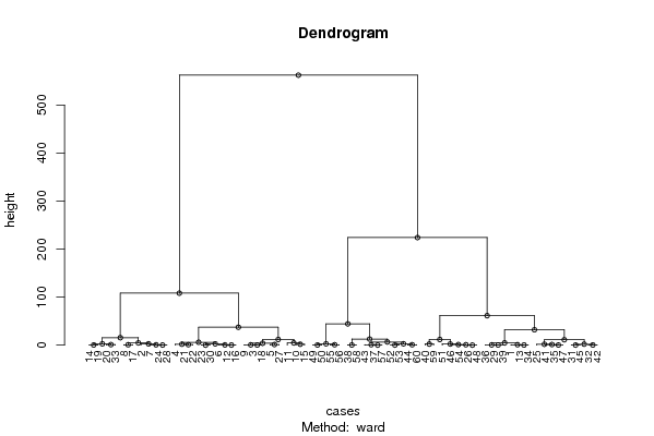
hc <- hclust(dist(x),method=par1)
d <- as.dendrogram(hc)
str(d)
mysub <- paste('Method: ',par1)
bitmap(file='test1.png')
if (par4 == 'TRUE'){
plot(d,main=main,ylab=ylab,xlab=xlab,horiz=par3, nodePar=list(pch = c(1,NA), cex=0.8, lab.cex = 0.8),type='t',center=T, sub=mysub)
} else {
plot(d,main=main,ylab=ylab,xlab=xlab,horiz=par3, nodePar=list(pch = c(1,NA), cex=0.8, lab.cex = 0.8), sub=mysub)
}
dev.off()
if (par2 != 'ALL'){
if (par3 == 'TRUE'){
ylab = 'cluster'
} else {
xlab = 'cluster'
}
par2 <- as.numeric(par2)
memb <- cutree(hc, k = par2)
cent <- NULL
for(k in 1:par2){
cent <- rbind(cent, colMeans(x[memb == k, , drop = FALSE]))
}
hc1 <- hclust(dist(cent),method=par1, members = table(memb))
de <- as.dendrogram(hc1)
bitmap(file='test2.png')
if (par4 == 'TRUE'){
plot(de,main=main,ylab=ylab,xlab=xlab,horiz=par3, nodePar=list(pch = c(1,NA), cex=0.8, lab.cex = 0.8),type='t',center=T, sub=mysub)
} else {
plot(de,main=main,ylab=ylab,xlab=xlab,horiz=par3, nodePar=list(pch = c(1,NA), cex=0.8, lab.cex = 0.8), sub=mysub)
}
dev.off()
str(de)
}
load(file='createtable')
a<-table.start()
a<-table.row.start(a)
a<-table.element(a,'Summary of Dendrogram',2,TRUE)
a<-table.row.end(a)
a<-table.row.start(a)
a<-table.element(a,'Label',header=TRUE)
a<-table.element(a,'Height',header=TRUE)
a<-table.row.end(a)
num <- length(x[,1])-1
for (i in 1:num)
{
a<-table.row.start(a)
a<-table.element(a,hc$labels[i])
a<-table.element(a,hc$height[i])
a<-table.row.end(a)
}
a<-table.end(a)
table.save(a,file='mytable1.tab')
if (par2 != 'ALL'){
a<-table.start()
a<-table.row.start(a)
a<-table.element(a,'Summary of Cut Dendrogram',2,TRUE)
a<-table.row.end(a)
a<-table.row.start(a)
a<-table.element(a,'Label',header=TRUE)
a<-table.element(a,'Height',header=TRUE)
a<-table.row.end(a)
num <- par2-1
for (i in 1:num)
{
a<-table.row.start(a)
a<-table.element(a,i)
a<-table.element(a,hc1$height[i])
a<-table.row.end(a)
}
a<-table.end(a)
table.save(a,file='mytable2.tab')
}

Free Statistics

Description of Statistical Computation

Tree of Dependent Computations

Dataset

Tables (Output of Computation)

Figures (Output of Computation)

Input Parameters & R Code