Repository of Reproducible Computations

Free Statistics

of Irreproducible Research!

Author's title

Author

*The author of this computation has been verified*

R Software Module

rwasp_autocorrelation.wasp

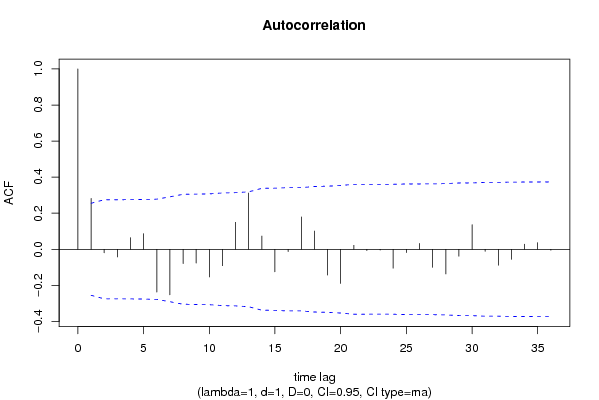
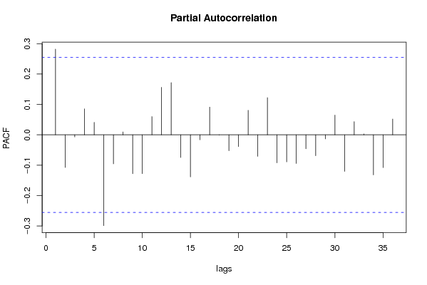
Title produced by software

(Partial) Autocorrelation Function

Date of computation

Wed, 02 Dec 2009 09:14:44 -0700

Cite this page as follows

Statistical Computations at FreeStatistics.org, Office for Research Development and Education, URL https://freestatistics.org/blog/index.php?v=date/2009/Dec/02/t1259770558ewf1ub5x37zphj5.htm/, Retrieved Sat, 27 Apr 2024 17:13:52 +0000

Statistical Computations at FreeStatistics.org, Office for Research Development and Education, URL https://freestatistics.org/blog/index.php?pk=62414, Retrieved Sat, 27 Apr 2024 17:13:52 +0000

QR Codes:

Paste this QR Code to cite your computation.

Original text written by user:

IsPrivate?

No (this computation is public)

User-defined keywords

Estimated Impact

173

Family? (F = Feedback message, R = changed R code, M = changed R Module, P = changed Parameters, D = changed Data)

-     [Univariate Explorative Data Analysis] [Run Sequence gebo...] [2008-12-12 13:32:37] [76963dc1903f0f612b6153510a3818cf]
- R  D  [Univariate Explorative Data Analysis] [Run Sequence gebo...] [2008-12-17 12:14:40] [76963dc1903f0f612b6153510a3818cf]
-         [Univariate Explorative Data Analysis] [Run Sequence Plot...] [2008-12-22 18:19:51] [1ce0d16c8f4225c977b42c8fa93bc163]
- RMP       [(Partial) Autocorrelation Function] [Identifying Integ...] [2009-11-22 12:16:10] [b98453cac15ba1066b407e146608df68]
-   PD        [(Partial) Autocorrelation Function] [WS8 d=1 D=1] [2009-11-25 16:19:15] [445b292c553470d9fed8bc2796fd3a00]
F   P             [(Partial) Autocorrelation Function] [WS8 autocorrelati...] [2009-12-02 16:14:44] [82f421ff86a0429b20e3ed68bd89f1bd] [Current]
-   P               [(Partial) Autocorrelation Function] [WS9] [2009-12-11 12:17:12] [4fe1472705bb0a32f118ba3ca90ffa8e] 
- RMP               [Standard Deviation-Mean Plot] [ws 9: Review 3] [2009-12-11 14:42:09] [b97b96148b0223bc16666763988dc147] 
- RMPD              [Spectral Analysis] [Spectrum D=0] [2010-01-07 15:15:02] [84dda5145c389bd11bcc662bd33fe4ba] 
-   P                 [Spectral Analysis] [Spectrum D=1] [2010-01-07 15:19:26] [84dda5145c389bd11bcc662bd33fe4ba] 
- R PD              [(Partial) Autocorrelation Function] [pacf ] [2010-01-07 15:26:43] [74be16979710d4c4e7c6647856088456] 
- RMPD              [ARIMA Backward Selection] [arima backwards p...] [2010-01-07 15:42:57] [74be16979710d4c4e7c6647856088456] 

Feedback Forum

2010-01-07 15:20:38 [Jef Keersmaekers] [reply] 
Beste, 
 
Er zijn enkele foutjes in je ws geslopen. In de vorige workshop werd bepaald dat de parameters voor jouw  
reeksen d=1 en D=0 moesten zijn. Dit kan op verschillende manieren worden getest. Via het spectrum kan je zien of je reeksen binnen het interval vallen.  
 
ik heb je reeks met je huidige waarden ingegeven in een spectrum 
http://www.freestatistics.org/blog/index.php?v=date/2010/Jan/07/t1262877354mx5lfp7qm0fmltg.htm/ 
als we het analyseren dan zien we dat de grafiek buiten het betrouwbaarheidsinterval valt. We moeten proberen dit binnen het interval laten vallen 
 
we zetten nu de D=1 en we zien nu dat de grafiek binnen het interval valt 
http://www.freestatistics.org/blog/index.php?v=date/2010/Jan/07/t1262877595imno0sgwd03p2so.htm/ 
 
Maw je gebruikte verkeerde waarden
2010-01-07 15:34:42 [Jef Keersmaekers] [reply] 
Dan voeren we onze waarden terug in om de partial correlation  te zoeken 
 
http://www.freestatistics.org/blog/index.php?v=date/2010/Jan/07/t1262878091bgis97lj9l2ne2x.htm/ 
 
in de bovenste grafiek een ligt patroon dat stil wegdeint naar het einde toe. we zien dus een patroon hier  
uit kunnen we uitmaken dat we al zeker een AR proces hebben. om te weten welke orde kijken we naar de onderstaande grafiek daar zijn geen outliers te bemerken. Dus besluiten we dat het een MA0 proces is.  
 
Als we dan de 2de grafiek bestuderen kunnen we ook stellen dat er een zeer licht patroon waarneembaar is. als we dan naar de bovenste grafiek kijken om de orde te bepalen zien we dat de 2de staaf bijna tegen het interval komt. We verlengen deze zodat we een MA proces verkrijgen
2010-01-07 15:38:45 [Jef Keersmaekers] [reply] 
We gaan nu op zoek naar onze waarden. 
 
p= aan het AR proces dit is 0 
p=0 
q= aan het maproces en dit is 1  
q=1 
P= seizoenaliteit op in de eerste grafiek er is er geen dus dit is 0 
P=0 
Q= seizonaliteit op de 2de grafiek dit is 0 
Q=0
  2010-01-07 15:43:38 [Jef Keersmaekers] [reply] 
Bij nader inzicht heb ik mij vergist en is het een AR 1 proces ipv AR0
2010-01-07 15:45:38 [Jef Keersmaekers] [reply] 
Nu gaan we deze waarden invullen in het arima backward proces 
http://www.freestatistics.org/blog/index.php?v=date/2010/Jan/07/t1262879078pcpng0s9j0dzefq.htm/ 
 
daaruit resulteren we dat een ma1 proces hebben

Post a new message

Dataseries X:

Download CSV

Histogram

Boxplots

7.55
7.55
7.59
7.59
7.59
7.57
7.57
7.59
7.6
7.64
7.64
7.76
7.76
7.76
7.77
7.83
7.94
7.94
7.94
8.09
8.18
8.26
8.28
8.28
8.28
8.29
8.3
8.3
8.31
8.33
8.33
8.34
8.48
8.59
8.67
8.67
8.67
8.71
8.72
8.72
8.72
8.74
8.74
8.74
8.74
8.79
8.85
8.86
8.87
8.92
8.96
8.97
8.99
8.98
8.98
9.01
9.01
9.03
9.05
9.05

Summary of computational transaction
Raw Input	view raw input (R code)
Raw Output	view raw output of R engine
Computing time	1 seconds
R Server	'Gwilym Jenkins' @ 72.249.127.135

\begin{tabular}{lllllllll}
\hline
Summary of computational transaction \tabularnewline
Raw Input & view raw input (R code)  \tabularnewline
Raw Output & view raw output of R engine  \tabularnewline
Computing time & 1 seconds \tabularnewline
R Server & 'Gwilym Jenkins' @ 72.249.127.135 \tabularnewline
\hline
\end{tabular}
%Source: https://freestatistics.org/blog/index.php?pk=62414&T=0

[TABLE]
[ROW][C]Summary of computational transaction[/C][/ROW]
[ROW][C]Raw Input[/C][C]view raw input (R code) [/C][/ROW]
[ROW][C]Raw Output[/C][C]view raw output of R engine [/C][/ROW]
[ROW][C]Computing time[/C][C]1 seconds[/C][/ROW]
[ROW][C]R Server[/C][C]'Gwilym Jenkins' @ 72.249.127.135[/C][/ROW]
[/TABLE]
Source: https://freestatistics.org/blog/index.php?pk=62414&T=0

Globally Unique Identifier (entire table): ba.freestatistics.org/blog/index.php?pk=62414&T=0

As an alternative you can also use a QR Code:

The GUIDs for individual cells are displayed in the table below:

Summary of computational transaction
Raw Input	view raw input (R code)
Raw Output	view raw output of R engine
Computing time	1 seconds
R Server	'Gwilym Jenkins' @ 72.249.127.135

Autocorrelation Function
Time lag k	ACF(k)	T-STAT	P-value
1	0.282109	2.1669	0.017145
2	-0.019514	-0.1499	0.440681
3	-0.042867	-0.3293	0.371559
4	0.06432	0.4941	0.311552
5	0.086183	0.662	0.255279
6	-0.237504	-1.8243	0.036586
7	-0.252311	-1.938	0.028704
8	-0.079086	-0.6075	0.272933
9	-0.07651	-0.5877	0.279493
10	-0.153625	-1.18	0.121364
11	-0.090877	-0.698	0.243946
12	0.149861	1.1511	0.127167
13	0.311529	2.3929	0.009959
14	0.073554	0.565	0.287114
15	-0.125264	-0.9622	0.169945
16	-0.012386	-0.0951	0.462264
17	0.179601	1.3795	0.086467
18	0.101146	0.7769	0.220156
19	-0.143219	-1.1001	0.137882
20	-0.189724	-1.4573	0.075168
21	0.022133	0.17	0.432794
22	-0.007474	-0.0574	0.477205
23	-0.004374	-0.0336	0.486657
24	-0.104602	-0.8035	0.212466
25	-0.018566	-0.1426	0.443542
26	0.032334	0.2484	0.402358
27	-0.10002	-0.7683	0.222697
28	-0.137066	-1.0528	0.148358
29	-0.038327	-0.2944	0.384744
30	0.136471	1.0483	0.149399
31	-0.011169	-0.0858	0.465962
32	-0.088323	-0.6784	0.250079
33	-0.055661	-0.4275	0.335272
34	0.028472	0.2187	0.413821
35	0.036584	0.281	0.389845
36	-0.005202	-0.04	0.484132

\begin{tabular}{lllllllll}
\hline
Autocorrelation Function \tabularnewline
Time lag k & ACF(k) & T-STAT & P-value \tabularnewline
1 & 0.282109 & 2.1669 & 0.017145 \tabularnewline
2 & -0.019514 & -0.1499 & 0.440681 \tabularnewline
3 & -0.042867 & -0.3293 & 0.371559 \tabularnewline
4 & 0.06432 & 0.4941 & 0.311552 \tabularnewline
5 & 0.086183 & 0.662 & 0.255279 \tabularnewline
6 & -0.237504 & -1.8243 & 0.036586 \tabularnewline
7 & -0.252311 & -1.938 & 0.028704 \tabularnewline
8 & -0.079086 & -0.6075 & 0.272933 \tabularnewline
9 & -0.07651 & -0.5877 & 0.279493 \tabularnewline
10 & -0.153625 & -1.18 & 0.121364 \tabularnewline
11 & -0.090877 & -0.698 & 0.243946 \tabularnewline
12 & 0.149861 & 1.1511 & 0.127167 \tabularnewline
13 & 0.311529 & 2.3929 & 0.009959 \tabularnewline
14 & 0.073554 & 0.565 & 0.287114 \tabularnewline
15 & -0.125264 & -0.9622 & 0.169945 \tabularnewline
16 & -0.012386 & -0.0951 & 0.462264 \tabularnewline
17 & 0.179601 & 1.3795 & 0.086467 \tabularnewline
18 & 0.101146 & 0.7769 & 0.220156 \tabularnewline
19 & -0.143219 & -1.1001 & 0.137882 \tabularnewline
20 & -0.189724 & -1.4573 & 0.075168 \tabularnewline
21 & 0.022133 & 0.17 & 0.432794 \tabularnewline
22 & -0.007474 & -0.0574 & 0.477205 \tabularnewline
23 & -0.004374 & -0.0336 & 0.486657 \tabularnewline
24 & -0.104602 & -0.8035 & 0.212466 \tabularnewline
25 & -0.018566 & -0.1426 & 0.443542 \tabularnewline
26 & 0.032334 & 0.2484 & 0.402358 \tabularnewline
27 & -0.10002 & -0.7683 & 0.222697 \tabularnewline
28 & -0.137066 & -1.0528 & 0.148358 \tabularnewline
29 & -0.038327 & -0.2944 & 0.384744 \tabularnewline
30 & 0.136471 & 1.0483 & 0.149399 \tabularnewline
31 & -0.011169 & -0.0858 & 0.465962 \tabularnewline
32 & -0.088323 & -0.6784 & 0.250079 \tabularnewline
33 & -0.055661 & -0.4275 & 0.335272 \tabularnewline
34 & 0.028472 & 0.2187 & 0.413821 \tabularnewline
35 & 0.036584 & 0.281 & 0.389845 \tabularnewline
36 & -0.005202 & -0.04 & 0.484132 \tabularnewline
\hline
\end{tabular}
%Source: https://freestatistics.org/blog/index.php?pk=62414&T=1

[TABLE]
[ROW][C]Autocorrelation Function[/C][/ROW]
[ROW][C]Time lag k[/C][C]ACF(k)[/C][C]T-STAT[/C][C]P-value[/C][/ROW]
[ROW][C]1[/C][C]0.282109[/C][C]2.1669[/C][C]0.017145[/C][/ROW]
[ROW][C]2[/C][C]-0.019514[/C][C]-0.1499[/C][C]0.440681[/C][/ROW]
[ROW][C]3[/C][C]-0.042867[/C][C]-0.3293[/C][C]0.371559[/C][/ROW]
[ROW][C]4[/C][C]0.06432[/C][C]0.4941[/C][C]0.311552[/C][/ROW]
[ROW][C]5[/C][C]0.086183[/C][C]0.662[/C][C]0.255279[/C][/ROW]
[ROW][C]6[/C][C]-0.237504[/C][C]-1.8243[/C][C]0.036586[/C][/ROW]
[ROW][C]7[/C][C]-0.252311[/C][C]-1.938[/C][C]0.028704[/C][/ROW]
[ROW][C]8[/C][C]-0.079086[/C][C]-0.6075[/C][C]0.272933[/C][/ROW]
[ROW][C]9[/C][C]-0.07651[/C][C]-0.5877[/C][C]0.279493[/C][/ROW]
[ROW][C]10[/C][C]-0.153625[/C][C]-1.18[/C][C]0.121364[/C][/ROW]
[ROW][C]11[/C][C]-0.090877[/C][C]-0.698[/C][C]0.243946[/C][/ROW]
[ROW][C]12[/C][C]0.149861[/C][C]1.1511[/C][C]0.127167[/C][/ROW]
[ROW][C]13[/C][C]0.311529[/C][C]2.3929[/C][C]0.009959[/C][/ROW]
[ROW][C]14[/C][C]0.073554[/C][C]0.565[/C][C]0.287114[/C][/ROW]
[ROW][C]15[/C][C]-0.125264[/C][C]-0.9622[/C][C]0.169945[/C][/ROW]
[ROW][C]16[/C][C]-0.012386[/C][C]-0.0951[/C][C]0.462264[/C][/ROW]
[ROW][C]17[/C][C]0.179601[/C][C]1.3795[/C][C]0.086467[/C][/ROW]
[ROW][C]18[/C][C]0.101146[/C][C]0.7769[/C][C]0.220156[/C][/ROW]
[ROW][C]19[/C][C]-0.143219[/C][C]-1.1001[/C][C]0.137882[/C][/ROW]
[ROW][C]20[/C][C]-0.189724[/C][C]-1.4573[/C][C]0.075168[/C][/ROW]
[ROW][C]21[/C][C]0.022133[/C][C]0.17[/C][C]0.432794[/C][/ROW]
[ROW][C]22[/C][C]-0.007474[/C][C]-0.0574[/C][C]0.477205[/C][/ROW]
[ROW][C]23[/C][C]-0.004374[/C][C]-0.0336[/C][C]0.486657[/C][/ROW]
[ROW][C]24[/C][C]-0.104602[/C][C]-0.8035[/C][C]0.212466[/C][/ROW]
[ROW][C]25[/C][C]-0.018566[/C][C]-0.1426[/C][C]0.443542[/C][/ROW]
[ROW][C]26[/C][C]0.032334[/C][C]0.2484[/C][C]0.402358[/C][/ROW]
[ROW][C]27[/C][C]-0.10002[/C][C]-0.7683[/C][C]0.222697[/C][/ROW]
[ROW][C]28[/C][C]-0.137066[/C][C]-1.0528[/C][C]0.148358[/C][/ROW]
[ROW][C]29[/C][C]-0.038327[/C][C]-0.2944[/C][C]0.384744[/C][/ROW]
[ROW][C]30[/C][C]0.136471[/C][C]1.0483[/C][C]0.149399[/C][/ROW]
[ROW][C]31[/C][C]-0.011169[/C][C]-0.0858[/C][C]0.465962[/C][/ROW]
[ROW][C]32[/C][C]-0.088323[/C][C]-0.6784[/C][C]0.250079[/C][/ROW]
[ROW][C]33[/C][C]-0.055661[/C][C]-0.4275[/C][C]0.335272[/C][/ROW]
[ROW][C]34[/C][C]0.028472[/C][C]0.2187[/C][C]0.413821[/C][/ROW]
[ROW][C]35[/C][C]0.036584[/C][C]0.281[/C][C]0.389845[/C][/ROW]
[ROW][C]36[/C][C]-0.005202[/C][C]-0.04[/C][C]0.484132[/C][/ROW]
[/TABLE]
Source: https://freestatistics.org/blog/index.php?pk=62414&T=1

Globally Unique Identifier (entire table): ba.freestatistics.org/blog/index.php?pk=62414&T=1

As an alternative you can also use a QR Code:

The GUIDs for individual cells are displayed in the table below:

Autocorrelation Function
Time lag k	ACF(k)	T-STAT	P-value
1	0.282109	2.1669	0.017145
2	-0.019514	-0.1499	0.440681
3	-0.042867	-0.3293	0.371559
4	0.06432	0.4941	0.311552
5	0.086183	0.662	0.255279
6	-0.237504	-1.8243	0.036586
7	-0.252311	-1.938	0.028704
8	-0.079086	-0.6075	0.272933
9	-0.07651	-0.5877	0.279493
10	-0.153625	-1.18	0.121364
11	-0.090877	-0.698	0.243946
12	0.149861	1.1511	0.127167
13	0.311529	2.3929	0.009959
14	0.073554	0.565	0.287114
15	-0.125264	-0.9622	0.169945
16	-0.012386	-0.0951	0.462264
17	0.179601	1.3795	0.086467
18	0.101146	0.7769	0.220156
19	-0.143219	-1.1001	0.137882
20	-0.189724	-1.4573	0.075168
21	0.022133	0.17	0.432794
22	-0.007474	-0.0574	0.477205
23	-0.004374	-0.0336	0.486657
24	-0.104602	-0.8035	0.212466
25	-0.018566	-0.1426	0.443542
26	0.032334	0.2484	0.402358
27	-0.10002	-0.7683	0.222697
28	-0.137066	-1.0528	0.148358
29	-0.038327	-0.2944	0.384744
30	0.136471	1.0483	0.149399
31	-0.011169	-0.0858	0.465962
32	-0.088323	-0.6784	0.250079
33	-0.055661	-0.4275	0.335272
34	0.028472	0.2187	0.413821
35	0.036584	0.281	0.389845
36	-0.005202	-0.04	0.484132

Partial Autocorrelation Function
Time lag k	PACF(k)	T-STAT	P-value
1	0.282109	2.1669	0.017145
2	-0.107668	-0.827	0.20578
3	-0.00703	-0.054	0.47856
4	0.085311	0.6553	0.257414
5	0.041232	0.3167	0.376292
6	-0.298922	-2.2961	0.012621
7	-0.095512	-0.7336	0.233037
8	0.009612	0.0738	0.470696
9	-0.127979	-0.983	0.164805
10	-0.127862	-0.9821	0.165024
11	0.060046	0.4612	0.323169
12	0.156468	1.2019	0.117111
13	0.171932	1.3206	0.095861
14	-0.074603	-0.573	0.284398
15	-0.138743	-1.0657	0.14545
16	-0.016422	-0.1261	0.450024
17	0.091284	0.7012	0.242978
18	-0.000925	-0.0071	0.497177
19	-0.052391	-0.4024	0.344412
20	-0.038765	-0.2978	0.383466
21	0.080806	0.6207	0.2686
22	-0.070852	-0.5442	0.294169
23	0.122222	0.9388	0.175829
24	-0.092325	-0.7092	0.240508
25	-0.088975	-0.6834	0.248506
26	-0.094431	-0.7253	0.235556
27	-0.046092	-0.354	0.362285
28	-0.068843	-0.5288	0.299466
29	-0.013483	-0.1036	0.458933
30	0.064975	0.4991	0.30979
31	-0.120522	-0.9257	0.179174
32	0.04337	0.3331	0.370108
33	0.003129	0.024	0.490454
34	-0.13179	-1.0123	0.157765
35	-0.107915	-0.8289	0.205248
36	0.051956	0.3991	0.345637

\begin{tabular}{lllllllll}
\hline
Partial Autocorrelation Function \tabularnewline
Time lag k & PACF(k) & T-STAT & P-value \tabularnewline
1 & 0.282109 & 2.1669 & 0.017145 \tabularnewline
2 & -0.107668 & -0.827 & 0.20578 \tabularnewline
3 & -0.00703 & -0.054 & 0.47856 \tabularnewline
4 & 0.085311 & 0.6553 & 0.257414 \tabularnewline
5 & 0.041232 & 0.3167 & 0.376292 \tabularnewline
6 & -0.298922 & -2.2961 & 0.012621 \tabularnewline
7 & -0.095512 & -0.7336 & 0.233037 \tabularnewline
8 & 0.009612 & 0.0738 & 0.470696 \tabularnewline
9 & -0.127979 & -0.983 & 0.164805 \tabularnewline
10 & -0.127862 & -0.9821 & 0.165024 \tabularnewline
11 & 0.060046 & 0.4612 & 0.323169 \tabularnewline
12 & 0.156468 & 1.2019 & 0.117111 \tabularnewline
13 & 0.171932 & 1.3206 & 0.095861 \tabularnewline
14 & -0.074603 & -0.573 & 0.284398 \tabularnewline
15 & -0.138743 & -1.0657 & 0.14545 \tabularnewline
16 & -0.016422 & -0.1261 & 0.450024 \tabularnewline
17 & 0.091284 & 0.7012 & 0.242978 \tabularnewline
18 & -0.000925 & -0.0071 & 0.497177 \tabularnewline
19 & -0.052391 & -0.4024 & 0.344412 \tabularnewline
20 & -0.038765 & -0.2978 & 0.383466 \tabularnewline
21 & 0.080806 & 0.6207 & 0.2686 \tabularnewline
22 & -0.070852 & -0.5442 & 0.294169 \tabularnewline
23 & 0.122222 & 0.9388 & 0.175829 \tabularnewline
24 & -0.092325 & -0.7092 & 0.240508 \tabularnewline
25 & -0.088975 & -0.6834 & 0.248506 \tabularnewline
26 & -0.094431 & -0.7253 & 0.235556 \tabularnewline
27 & -0.046092 & -0.354 & 0.362285 \tabularnewline
28 & -0.068843 & -0.5288 & 0.299466 \tabularnewline
29 & -0.013483 & -0.1036 & 0.458933 \tabularnewline
30 & 0.064975 & 0.4991 & 0.30979 \tabularnewline
31 & -0.120522 & -0.9257 & 0.179174 \tabularnewline
32 & 0.04337 & 0.3331 & 0.370108 \tabularnewline
33 & 0.003129 & 0.024 & 0.490454 \tabularnewline
34 & -0.13179 & -1.0123 & 0.157765 \tabularnewline
35 & -0.107915 & -0.8289 & 0.205248 \tabularnewline
36 & 0.051956 & 0.3991 & 0.345637 \tabularnewline
\hline
\end{tabular}
%Source: https://freestatistics.org/blog/index.php?pk=62414&T=2

[TABLE]
[ROW][C]Partial Autocorrelation Function[/C][/ROW]
[ROW][C]Time lag k[/C][C]PACF(k)[/C][C]T-STAT[/C][C]P-value[/C][/ROW]
[ROW][C]1[/C][C]0.282109[/C][C]2.1669[/C][C]0.017145[/C][/ROW]
[ROW][C]2[/C][C]-0.107668[/C][C]-0.827[/C][C]0.20578[/C][/ROW]
[ROW][C]3[/C][C]-0.00703[/C][C]-0.054[/C][C]0.47856[/C][/ROW]
[ROW][C]4[/C][C]0.085311[/C][C]0.6553[/C][C]0.257414[/C][/ROW]
[ROW][C]5[/C][C]0.041232[/C][C]0.3167[/C][C]0.376292[/C][/ROW]
[ROW][C]6[/C][C]-0.298922[/C][C]-2.2961[/C][C]0.012621[/C][/ROW]
[ROW][C]7[/C][C]-0.095512[/C][C]-0.7336[/C][C]0.233037[/C][/ROW]
[ROW][C]8[/C][C]0.009612[/C][C]0.0738[/C][C]0.470696[/C][/ROW]
[ROW][C]9[/C][C]-0.127979[/C][C]-0.983[/C][C]0.164805[/C][/ROW]
[ROW][C]10[/C][C]-0.127862[/C][C]-0.9821[/C][C]0.165024[/C][/ROW]
[ROW][C]11[/C][C]0.060046[/C][C]0.4612[/C][C]0.323169[/C][/ROW]
[ROW][C]12[/C][C]0.156468[/C][C]1.2019[/C][C]0.117111[/C][/ROW]
[ROW][C]13[/C][C]0.171932[/C][C]1.3206[/C][C]0.095861[/C][/ROW]
[ROW][C]14[/C][C]-0.074603[/C][C]-0.573[/C][C]0.284398[/C][/ROW]
[ROW][C]15[/C][C]-0.138743[/C][C]-1.0657[/C][C]0.14545[/C][/ROW]
[ROW][C]16[/C][C]-0.016422[/C][C]-0.1261[/C][C]0.450024[/C][/ROW]
[ROW][C]17[/C][C]0.091284[/C][C]0.7012[/C][C]0.242978[/C][/ROW]
[ROW][C]18[/C][C]-0.000925[/C][C]-0.0071[/C][C]0.497177[/C][/ROW]
[ROW][C]19[/C][C]-0.052391[/C][C]-0.4024[/C][C]0.344412[/C][/ROW]
[ROW][C]20[/C][C]-0.038765[/C][C]-0.2978[/C][C]0.383466[/C][/ROW]
[ROW][C]21[/C][C]0.080806[/C][C]0.6207[/C][C]0.2686[/C][/ROW]
[ROW][C]22[/C][C]-0.070852[/C][C]-0.5442[/C][C]0.294169[/C][/ROW]
[ROW][C]23[/C][C]0.122222[/C][C]0.9388[/C][C]0.175829[/C][/ROW]
[ROW][C]24[/C][C]-0.092325[/C][C]-0.7092[/C][C]0.240508[/C][/ROW]
[ROW][C]25[/C][C]-0.088975[/C][C]-0.6834[/C][C]0.248506[/C][/ROW]
[ROW][C]26[/C][C]-0.094431[/C][C]-0.7253[/C][C]0.235556[/C][/ROW]
[ROW][C]27[/C][C]-0.046092[/C][C]-0.354[/C][C]0.362285[/C][/ROW]
[ROW][C]28[/C][C]-0.068843[/C][C]-0.5288[/C][C]0.299466[/C][/ROW]
[ROW][C]29[/C][C]-0.013483[/C][C]-0.1036[/C][C]0.458933[/C][/ROW]
[ROW][C]30[/C][C]0.064975[/C][C]0.4991[/C][C]0.30979[/C][/ROW]
[ROW][C]31[/C][C]-0.120522[/C][C]-0.9257[/C][C]0.179174[/C][/ROW]
[ROW][C]32[/C][C]0.04337[/C][C]0.3331[/C][C]0.370108[/C][/ROW]
[ROW][C]33[/C][C]0.003129[/C][C]0.024[/C][C]0.490454[/C][/ROW]
[ROW][C]34[/C][C]-0.13179[/C][C]-1.0123[/C][C]0.157765[/C][/ROW]
[ROW][C]35[/C][C]-0.107915[/C][C]-0.8289[/C][C]0.205248[/C][/ROW]
[ROW][C]36[/C][C]0.051956[/C][C]0.3991[/C][C]0.345637[/C][/ROW]
[/TABLE]
Source: https://freestatistics.org/blog/index.php?pk=62414&T=2

Globally Unique Identifier (entire table): ba.freestatistics.org/blog/index.php?pk=62414&T=2

As an alternative you can also use a QR Code:

The GUIDs for individual cells are displayed in the table below:

Partial Autocorrelation Function
Time lag k	PACF(k)	T-STAT	P-value
1	0.282109	2.1669	0.017145
2	-0.107668	-0.827	0.20578
3	-0.00703	-0.054	0.47856
4	0.085311	0.6553	0.257414
5	0.041232	0.3167	0.376292
6	-0.298922	-2.2961	0.012621
7	-0.095512	-0.7336	0.233037
8	0.009612	0.0738	0.470696
9	-0.127979	-0.983	0.164805
10	-0.127862	-0.9821	0.165024
11	0.060046	0.4612	0.323169
12	0.156468	1.2019	0.117111
13	0.171932	1.3206	0.095861
14	-0.074603	-0.573	0.284398
15	-0.138743	-1.0657	0.14545
16	-0.016422	-0.1261	0.450024
17	0.091284	0.7012	0.242978
18	-0.000925	-0.0071	0.497177
19	-0.052391	-0.4024	0.344412
20	-0.038765	-0.2978	0.383466
21	0.080806	0.6207	0.2686
22	-0.070852	-0.5442	0.294169
23	0.122222	0.9388	0.175829
24	-0.092325	-0.7092	0.240508
25	-0.088975	-0.6834	0.248506
26	-0.094431	-0.7253	0.235556
27	-0.046092	-0.354	0.362285
28	-0.068843	-0.5288	0.299466
29	-0.013483	-0.1036	0.458933
30	0.064975	0.4991	0.30979
31	-0.120522	-0.9257	0.179174
32	0.04337	0.3331	0.370108
33	0.003129	0.024	0.490454
34	-0.13179	-1.0123	0.157765
35	-0.107915	-0.8289	0.205248
36	0.051956	0.3991	0.345637

Figure 1

PNG link

Postscript link

PDF link

Figure 2

PNG link

Postscript link

PDF link

Parameters (Session):

par1 = 36 ; par2 = 1 ; par3 = 1 ; par4 = 0 ; par5 = 12 ; par6 = MA ; par7 = 0.95 ;

Parameters (R input):

par1 = 36 ; par2 = 1 ; par3 = 1 ; par4 = 0 ; par5 = 12 ; par6 = MA ; par7 = 0.95 ;

R code (references can be found in the software module):

if (par1 == 'Default') {
par1 = 10*log10(length(x))
} else {
par1 <- as.numeric(par1)
}
par2 <- as.numeric(par2)
par3 <- as.numeric(par3)
par4 <- as.numeric(par4)
par5 <- as.numeric(par5)
if (par6 == 'White Noise') par6 <- 'white' else par6 <- 'ma'
par7 <- as.numeric(par7)
if (par2 == 0) {
x <- log(x)
} else {
x <- (x ^ par2 - 1) / par2
}
if (par3 > 0) x <- diff(x,lag=1,difference=par3)
if (par4 > 0) x <- diff(x,lag=par5,difference=par4)
bitmap(file='pic1.png')
racf <- acf(x, par1, main='Autocorrelation', xlab='time lag', ylab='ACF', ci.type=par6, ci=par7, sub=paste('(lambda=',par2,', d=',par3,', D=',par4,', CI=', par7, ', CI type=',par6,')',sep=''))
dev.off()
bitmap(file='pic2.png')
rpacf <- pacf(x,par1,main='Partial Autocorrelation',xlab='lags',ylab='PACF')
dev.off()
(myacf <- c(racf$acf))
(mypacf <- c(rpacf$acf))
lengthx <- length(x)
sqrtn <- sqrt(lengthx)
load(file='createtable')
a<-table.start()
a<-table.row.start(a)
a<-table.element(a,'Autocorrelation Function',4,TRUE)
a<-table.row.end(a)
a<-table.row.start(a)
a<-table.element(a,'Time lag k',header=TRUE)
a<-table.element(a,hyperlink('basics.htm','ACF(k)','click here for more information about the Autocorrelation Function'),header=TRUE)
a<-table.element(a,'T-STAT',header=TRUE)
a<-table.element(a,'P-value',header=TRUE)
a<-table.row.end(a)
for (i in 2:(par1+1)) {
a<-table.row.start(a)
a<-table.element(a,i-1,header=TRUE)
a<-table.element(a,round(myacf[i],6))
mytstat <- myacf[i]*sqrtn
a<-table.element(a,round(mytstat,4))
a<-table.element(a,round(1-pt(abs(mytstat),lengthx),6))
a<-table.row.end(a)
}
a<-table.end(a)
table.save(a,file='mytable.tab')
a<-table.start()
a<-table.row.start(a)
a<-table.element(a,'Partial Autocorrelation Function',4,TRUE)
a<-table.row.end(a)
a<-table.row.start(a)
a<-table.element(a,'Time lag k',header=TRUE)
a<-table.element(a,hyperlink('basics.htm','PACF(k)','click here for more information about the Partial Autocorrelation Function'),header=TRUE)
a<-table.element(a,'T-STAT',header=TRUE)
a<-table.element(a,'P-value',header=TRUE)
a<-table.row.end(a)
for (i in 1:par1) {
a<-table.row.start(a)
a<-table.element(a,i,header=TRUE)
a<-table.element(a,round(mypacf[i],6))
mytstat <- mypacf[i]*sqrtn
a<-table.element(a,round(mytstat,4))
a<-table.element(a,round(1-pt(abs(mytstat),lengthx),6))
a<-table.row.end(a)
}
a<-table.end(a)
table.save(a,file='mytable1.tab')

Free Statistics

Description of Statistical Computation

Tree of Dependent Computations

Dataset

Tables (Output of Computation)

Figures (Output of Computation)

Input Parameters & R Code