Repository of Reproducible Computations

Free Statistics

of Irreproducible Research!

Author's title

Author

*The author of this computation has been verified*

R Software Module

rwasp_autocorrelation.wasp

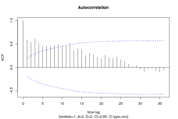
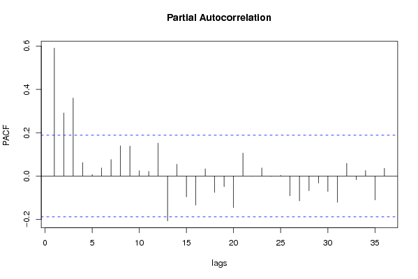
Title produced by software

(Partial) Autocorrelation Function

Date of computation

Fri, 04 Dec 2009 08:13:05 -0700

Cite this page as follows

Statistical Computations at FreeStatistics.org, Office for Research Development and Education, URL https://freestatistics.org/blog/index.php?v=date/2009/Dec/04/t1259939615bj3c6f4nm9uo8kz.htm/, Retrieved Sun, 28 Apr 2024 10:33:28 +0000

Statistical Computations at FreeStatistics.org, Office for Research Development and Education, URL https://freestatistics.org/blog/index.php?pk=63731, Retrieved Sun, 28 Apr 2024 10:33:28 +0000

QR Codes:

Paste this QR Code to cite your computation.

Original text written by user:

IsPrivate?

No (this computation is public)

User-defined keywords

Estimated Impact

114

Family? (F = Feedback message, R = changed R code, M = changed R Module, P = changed Parameters, D = changed Data)

-     [Univariate Explorative Data Analysis] [Run Sequence gebo...] [2008-12-12 13:32:37] [76963dc1903f0f612b6153510a3818cf]
- R  D  [Univariate Explorative Data Analysis] [Run Sequence gebo...] [2008-12-17 12:14:40] [76963dc1903f0f612b6153510a3818cf]
-         [Univariate Explorative Data Analysis] [Run Sequence Plot...] [2008-12-22 18:19:51] [1ce0d16c8f4225c977b42c8fa93bc163]
- RMP       [(Partial) Autocorrelation Function] [Identifying Integ...] [2009-11-22 12:16:10] [b98453cac15ba1066b407e146608df68]
-   PD        [(Partial) Autocorrelation Function] [Bouwvergunningen ...] [2009-11-27 14:23:36] [11ac052cc87d77b9933b02bea117068e]
-   P           [(Partial) Autocorrelation Function] [Bouwvergunningen ...] [2009-11-27 14:34:47] [11ac052cc87d77b9933b02bea117068e]
- R  D              [(Partial) Autocorrelation Function] [] [2009-12-04 15:13:05] [2795ec65528c1a16d9df20713e7edc71] [Current]

Feedback Forum

Post a new message

Dataseries X:

Download CSV

Histogram

Boxplots

100
108,1560276
114,0150276
102,1880309
110,3672031
96,8602511
94,1944583
99,51621961
94,06333487
97,5541476
78,15062422
81,2434643
92,36262465
96,06324371
114,0523777
110,6616666
104,9171949
90,00187193
95,7008067
86,02741157
84,85287668
100,04328
80,91713823
74,06539709
77,30281369
97,23043249
90,75515676
100,5614455
92,01293267
99,24012138
105,8672755
90,9920463
93,30624423
91,17419413
77,33295039
91,1277721
85,01249943
83,90390242
104,8626302
110,9039108
95,43714373
111,6238727
108,8925403
96,17511682
101,9740205
99,11953031
86,78158147
118,4195003
118,7441447
106,5296192
134,7772694
104,6778714
105,2954304
139,4139849
103,6060491
99,78182974
103,4610301
120,0594945
96,71377168
107,1308929
105,3608372
111,6942359
132,0519998
126,8037879
154,4824253
141,5570984
109,9506882
127,904198
133,0888617
120,0796299
117,5557142
143,0362309
159,982927
128,5991124
149,7373327
126,8169313
140,9639674
137,6691981
117,9402337
122,3095247
127,7804207
136,1677176
116,2405856
123,1576893
116,3400234
108,6119282
125,8982264
112,8003105
107,5182447
135,0955413
115,5096488
115,8640759
104,5883906
163,7213386
113,4482275
98,0428844
116,7868521
126,5330444
113,0336597
124,3392163
109,8298759
124,4434777
111,5039454
102,0350019
116,8726598
112,2073122
101,1513902
124,4255108

Summary of computational transaction
Raw Input	view raw input (R code)
Raw Output	view raw output of R engine
Computing time	1 seconds
R Server	'Gwilym Jenkins' @ 72.249.127.135

\begin{tabular}{lllllllll}
\hline
Summary of computational transaction \tabularnewline
Raw Input & view raw input (R code)  \tabularnewline
Raw Output & view raw output of R engine  \tabularnewline
Computing time & 1 seconds \tabularnewline
R Server & 'Gwilym Jenkins' @ 72.249.127.135 \tabularnewline
\hline
\end{tabular}
%Source: https://freestatistics.org/blog/index.php?pk=63731&T=0

[TABLE]
[ROW][C]Summary of computational transaction[/C][/ROW]
[ROW][C]Raw Input[/C][C]view raw input (R code) [/C][/ROW]
[ROW][C]Raw Output[/C][C]view raw output of R engine [/C][/ROW]
[ROW][C]Computing time[/C][C]1 seconds[/C][/ROW]
[ROW][C]R Server[/C][C]'Gwilym Jenkins' @ 72.249.127.135[/C][/ROW]
[/TABLE]
Source: https://freestatistics.org/blog/index.php?pk=63731&T=0

Globally Unique Identifier (entire table): ba.freestatistics.org/blog/index.php?pk=63731&T=0

As an alternative you can also use a QR Code:

The GUIDs for individual cells are displayed in the table below:

Summary of computational transaction
Raw Input	view raw input (R code)
Raw Output	view raw output of R engine
Computing time	1 seconds
R Server	'Gwilym Jenkins' @ 72.249.127.135

Autocorrelation Function
Time lag k	ACF(k)	T-STAT	P-value
1	0.590909	6.1409	0
2	0.538779	5.5992	0
3	0.612348	6.3637	0
4	0.513008	5.3313	0
5	0.453966	4.7178	4e-06
6	0.462266	4.804	3e-06
7	0.452982	4.7075	4e-06
8	0.467794	4.8615	2e-06
9	0.488013	5.0716	1e-06
10	0.452228	4.6997	4e-06
11	0.452211	4.6995	4e-06
12	0.520174	5.4058	0
13	0.352577	3.6641	0.000193
14	0.398743	4.1439	3.4e-05
15	0.374705	3.894	8.6e-05
16	0.257682	2.6779	0.004283
17	0.306104	3.1811	0.000958
18	0.272249	2.8293	0.002781
19	0.219557	2.2817	0.012234
20	0.187387	1.9474	0.027042
21	0.261484	2.7174	0.003833
22	0.217515	2.2605	0.012898
23	0.200221	2.0808	0.019911
24	0.223714	2.3249	0.010973
25	0.167705	1.7428	0.042104
26	0.139325	1.4479	0.075269
27	0.072301	0.7514	0.227031
28	0.01519	0.1579	0.43743
29	0.042769	0.4445	0.328796
30	-0.040407	-0.4199	0.337687
31	-0.084275	-0.8758	0.191539
32	-0.030087	-0.3127	0.377565
33	-0.022968	-0.2387	0.405898
34	-0.070805	-0.7358	0.231714
35	-0.096881	-1.0068	0.158137
36	-0.055853	-0.5804	0.281413

\begin{tabular}{lllllllll}
\hline
Autocorrelation Function \tabularnewline
Time lag k & ACF(k) & T-STAT & P-value \tabularnewline
1 & 0.590909 & 6.1409 & 0 \tabularnewline
2 & 0.538779 & 5.5992 & 0 \tabularnewline
3 & 0.612348 & 6.3637 & 0 \tabularnewline
4 & 0.513008 & 5.3313 & 0 \tabularnewline
5 & 0.453966 & 4.7178 & 4e-06 \tabularnewline
6 & 0.462266 & 4.804 & 3e-06 \tabularnewline
7 & 0.452982 & 4.7075 & 4e-06 \tabularnewline
8 & 0.467794 & 4.8615 & 2e-06 \tabularnewline
9 & 0.488013 & 5.0716 & 1e-06 \tabularnewline
10 & 0.452228 & 4.6997 & 4e-06 \tabularnewline
11 & 0.452211 & 4.6995 & 4e-06 \tabularnewline
12 & 0.520174 & 5.4058 & 0 \tabularnewline
13 & 0.352577 & 3.6641 & 0.000193 \tabularnewline
14 & 0.398743 & 4.1439 & 3.4e-05 \tabularnewline
15 & 0.374705 & 3.894 & 8.6e-05 \tabularnewline
16 & 0.257682 & 2.6779 & 0.004283 \tabularnewline
17 & 0.306104 & 3.1811 & 0.000958 \tabularnewline
18 & 0.272249 & 2.8293 & 0.002781 \tabularnewline
19 & 0.219557 & 2.2817 & 0.012234 \tabularnewline
20 & 0.187387 & 1.9474 & 0.027042 \tabularnewline
21 & 0.261484 & 2.7174 & 0.003833 \tabularnewline
22 & 0.217515 & 2.2605 & 0.012898 \tabularnewline
23 & 0.200221 & 2.0808 & 0.019911 \tabularnewline
24 & 0.223714 & 2.3249 & 0.010973 \tabularnewline
25 & 0.167705 & 1.7428 & 0.042104 \tabularnewline
26 & 0.139325 & 1.4479 & 0.075269 \tabularnewline
27 & 0.072301 & 0.7514 & 0.227031 \tabularnewline
28 & 0.01519 & 0.1579 & 0.43743 \tabularnewline
29 & 0.042769 & 0.4445 & 0.328796 \tabularnewline
30 & -0.040407 & -0.4199 & 0.337687 \tabularnewline
31 & -0.084275 & -0.8758 & 0.191539 \tabularnewline
32 & -0.030087 & -0.3127 & 0.377565 \tabularnewline
33 & -0.022968 & -0.2387 & 0.405898 \tabularnewline
34 & -0.070805 & -0.7358 & 0.231714 \tabularnewline
35 & -0.096881 & -1.0068 & 0.158137 \tabularnewline
36 & -0.055853 & -0.5804 & 0.281413 \tabularnewline
\hline
\end{tabular}
%Source: https://freestatistics.org/blog/index.php?pk=63731&T=1

[TABLE]
[ROW][C]Autocorrelation Function[/C][/ROW]
[ROW][C]Time lag k[/C][C]ACF(k)[/C][C]T-STAT[/C][C]P-value[/C][/ROW]
[ROW][C]1[/C][C]0.590909[/C][C]6.1409[/C][C]0[/C][/ROW]
[ROW][C]2[/C][C]0.538779[/C][C]5.5992[/C][C]0[/C][/ROW]
[ROW][C]3[/C][C]0.612348[/C][C]6.3637[/C][C]0[/C][/ROW]
[ROW][C]4[/C][C]0.513008[/C][C]5.3313[/C][C]0[/C][/ROW]
[ROW][C]5[/C][C]0.453966[/C][C]4.7178[/C][C]4e-06[/C][/ROW]
[ROW][C]6[/C][C]0.462266[/C][C]4.804[/C][C]3e-06[/C][/ROW]
[ROW][C]7[/C][C]0.452982[/C][C]4.7075[/C][C]4e-06[/C][/ROW]
[ROW][C]8[/C][C]0.467794[/C][C]4.8615[/C][C]2e-06[/C][/ROW]
[ROW][C]9[/C][C]0.488013[/C][C]5.0716[/C][C]1e-06[/C][/ROW]
[ROW][C]10[/C][C]0.452228[/C][C]4.6997[/C][C]4e-06[/C][/ROW]
[ROW][C]11[/C][C]0.452211[/C][C]4.6995[/C][C]4e-06[/C][/ROW]
[ROW][C]12[/C][C]0.520174[/C][C]5.4058[/C][C]0[/C][/ROW]
[ROW][C]13[/C][C]0.352577[/C][C]3.6641[/C][C]0.000193[/C][/ROW]
[ROW][C]14[/C][C]0.398743[/C][C]4.1439[/C][C]3.4e-05[/C][/ROW]
[ROW][C]15[/C][C]0.374705[/C][C]3.894[/C][C]8.6e-05[/C][/ROW]
[ROW][C]16[/C][C]0.257682[/C][C]2.6779[/C][C]0.004283[/C][/ROW]
[ROW][C]17[/C][C]0.306104[/C][C]3.1811[/C][C]0.000958[/C][/ROW]
[ROW][C]18[/C][C]0.272249[/C][C]2.8293[/C][C]0.002781[/C][/ROW]
[ROW][C]19[/C][C]0.219557[/C][C]2.2817[/C][C]0.012234[/C][/ROW]
[ROW][C]20[/C][C]0.187387[/C][C]1.9474[/C][C]0.027042[/C][/ROW]
[ROW][C]21[/C][C]0.261484[/C][C]2.7174[/C][C]0.003833[/C][/ROW]
[ROW][C]22[/C][C]0.217515[/C][C]2.2605[/C][C]0.012898[/C][/ROW]
[ROW][C]23[/C][C]0.200221[/C][C]2.0808[/C][C]0.019911[/C][/ROW]
[ROW][C]24[/C][C]0.223714[/C][C]2.3249[/C][C]0.010973[/C][/ROW]
[ROW][C]25[/C][C]0.167705[/C][C]1.7428[/C][C]0.042104[/C][/ROW]
[ROW][C]26[/C][C]0.139325[/C][C]1.4479[/C][C]0.075269[/C][/ROW]
[ROW][C]27[/C][C]0.072301[/C][C]0.7514[/C][C]0.227031[/C][/ROW]
[ROW][C]28[/C][C]0.01519[/C][C]0.1579[/C][C]0.43743[/C][/ROW]
[ROW][C]29[/C][C]0.042769[/C][C]0.4445[/C][C]0.328796[/C][/ROW]
[ROW][C]30[/C][C]-0.040407[/C][C]-0.4199[/C][C]0.337687[/C][/ROW]
[ROW][C]31[/C][C]-0.084275[/C][C]-0.8758[/C][C]0.191539[/C][/ROW]
[ROW][C]32[/C][C]-0.030087[/C][C]-0.3127[/C][C]0.377565[/C][/ROW]
[ROW][C]33[/C][C]-0.022968[/C][C]-0.2387[/C][C]0.405898[/C][/ROW]
[ROW][C]34[/C][C]-0.070805[/C][C]-0.7358[/C][C]0.231714[/C][/ROW]
[ROW][C]35[/C][C]-0.096881[/C][C]-1.0068[/C][C]0.158137[/C][/ROW]
[ROW][C]36[/C][C]-0.055853[/C][C]-0.5804[/C][C]0.281413[/C][/ROW]
[/TABLE]
Source: https://freestatistics.org/blog/index.php?pk=63731&T=1

Globally Unique Identifier (entire table): ba.freestatistics.org/blog/index.php?pk=63731&T=1

As an alternative you can also use a QR Code:

The GUIDs for individual cells are displayed in the table below:

Autocorrelation Function
Time lag k	ACF(k)	T-STAT	P-value
1	0.590909	6.1409	0
2	0.538779	5.5992	0
3	0.612348	6.3637	0
4	0.513008	5.3313	0
5	0.453966	4.7178	4e-06
6	0.462266	4.804	3e-06
7	0.452982	4.7075	4e-06
8	0.467794	4.8615	2e-06
9	0.488013	5.0716	1e-06
10	0.452228	4.6997	4e-06
11	0.452211	4.6995	4e-06
12	0.520174	5.4058	0
13	0.352577	3.6641	0.000193
14	0.398743	4.1439	3.4e-05
15	0.374705	3.894	8.6e-05
16	0.257682	2.6779	0.004283
17	0.306104	3.1811	0.000958
18	0.272249	2.8293	0.002781
19	0.219557	2.2817	0.012234
20	0.187387	1.9474	0.027042
21	0.261484	2.7174	0.003833
22	0.217515	2.2605	0.012898
23	0.200221	2.0808	0.019911
24	0.223714	2.3249	0.010973
25	0.167705	1.7428	0.042104
26	0.139325	1.4479	0.075269
27	0.072301	0.7514	0.227031
28	0.01519	0.1579	0.43743
29	0.042769	0.4445	0.328796
30	-0.040407	-0.4199	0.337687
31	-0.084275	-0.8758	0.191539
32	-0.030087	-0.3127	0.377565
33	-0.022968	-0.2387	0.405898
34	-0.070805	-0.7358	0.231714
35	-0.096881	-1.0068	0.158137
36	-0.055853	-0.5804	0.281413

Partial Autocorrelation Function
Time lag k	PACF(k)	T-STAT	P-value
1	0.590909	6.1409	0
2	0.29133	3.0276	0.001542
3	0.360282	3.7442	0.000146
4	0.062291	0.6473	0.259391
5	0.006696	0.0696	0.472324
6	0.037223	0.3868	0.349821
7	0.076124	0.7911	0.215308
8	0.139466	1.4494	0.075066
9	0.138121	1.4354	0.077032
10	0.024218	0.2517	0.400884
11	0.021316	0.2215	0.412554
12	0.151726	1.5768	0.058885
13	-0.207255	-2.1539	0.016737
14	0.054607	0.5675	0.285779
15	-0.096124	-0.9989	0.160026
16	-0.134509	-1.3979	0.08251
17	0.033016	0.3431	0.366091
18	-0.075574	-0.7854	0.216972
19	-0.048933	-0.5085	0.306062
20	-0.145945	-1.5167	0.066131
21	0.105599	1.0974	0.137449
22	2e-06	0	0.499994
23	0.03703	0.3848	0.350563
24	-0.001691	-0.0176	0.493004
25	0.003044	0.0316	0.48741
26	-0.09119	-0.9477	0.172704
27	-0.115	-1.1951	0.117329
28	-0.06783	-0.7049	0.241193
29	-0.032797	-0.3408	0.366944
30	-0.071212	-0.7401	0.230434
31	-0.121585	-1.2635	0.104556
32	0.058653	0.6095	0.271725
33	-0.017464	-0.1815	0.42816
34	0.025133	0.2612	0.397221
35	-0.110618	-1.1496	0.126429
36	0.035855	0.3726	0.355082

\begin{tabular}{lllllllll}
\hline
Partial Autocorrelation Function \tabularnewline
Time lag k & PACF(k) & T-STAT & P-value \tabularnewline
1 & 0.590909 & 6.1409 & 0 \tabularnewline
2 & 0.29133 & 3.0276 & 0.001542 \tabularnewline
3 & 0.360282 & 3.7442 & 0.000146 \tabularnewline
4 & 0.062291 & 0.6473 & 0.259391 \tabularnewline
5 & 0.006696 & 0.0696 & 0.472324 \tabularnewline
6 & 0.037223 & 0.3868 & 0.349821 \tabularnewline
7 & 0.076124 & 0.7911 & 0.215308 \tabularnewline
8 & 0.139466 & 1.4494 & 0.075066 \tabularnewline
9 & 0.138121 & 1.4354 & 0.077032 \tabularnewline
10 & 0.024218 & 0.2517 & 0.400884 \tabularnewline
11 & 0.021316 & 0.2215 & 0.412554 \tabularnewline
12 & 0.151726 & 1.5768 & 0.058885 \tabularnewline
13 & -0.207255 & -2.1539 & 0.016737 \tabularnewline
14 & 0.054607 & 0.5675 & 0.285779 \tabularnewline
15 & -0.096124 & -0.9989 & 0.160026 \tabularnewline
16 & -0.134509 & -1.3979 & 0.08251 \tabularnewline
17 & 0.033016 & 0.3431 & 0.366091 \tabularnewline
18 & -0.075574 & -0.7854 & 0.216972 \tabularnewline
19 & -0.048933 & -0.5085 & 0.306062 \tabularnewline
20 & -0.145945 & -1.5167 & 0.066131 \tabularnewline
21 & 0.105599 & 1.0974 & 0.137449 \tabularnewline
22 & 2e-06 & 0 & 0.499994 \tabularnewline
23 & 0.03703 & 0.3848 & 0.350563 \tabularnewline
24 & -0.001691 & -0.0176 & 0.493004 \tabularnewline
25 & 0.003044 & 0.0316 & 0.48741 \tabularnewline
26 & -0.09119 & -0.9477 & 0.172704 \tabularnewline
27 & -0.115 & -1.1951 & 0.117329 \tabularnewline
28 & -0.06783 & -0.7049 & 0.241193 \tabularnewline
29 & -0.032797 & -0.3408 & 0.366944 \tabularnewline
30 & -0.071212 & -0.7401 & 0.230434 \tabularnewline
31 & -0.121585 & -1.2635 & 0.104556 \tabularnewline
32 & 0.058653 & 0.6095 & 0.271725 \tabularnewline
33 & -0.017464 & -0.1815 & 0.42816 \tabularnewline
34 & 0.025133 & 0.2612 & 0.397221 \tabularnewline
35 & -0.110618 & -1.1496 & 0.126429 \tabularnewline
36 & 0.035855 & 0.3726 & 0.355082 \tabularnewline
\hline
\end{tabular}
%Source: https://freestatistics.org/blog/index.php?pk=63731&T=2

[TABLE]
[ROW][C]Partial Autocorrelation Function[/C][/ROW]
[ROW][C]Time lag k[/C][C]PACF(k)[/C][C]T-STAT[/C][C]P-value[/C][/ROW]
[ROW][C]1[/C][C]0.590909[/C][C]6.1409[/C][C]0[/C][/ROW]
[ROW][C]2[/C][C]0.29133[/C][C]3.0276[/C][C]0.001542[/C][/ROW]
[ROW][C]3[/C][C]0.360282[/C][C]3.7442[/C][C]0.000146[/C][/ROW]
[ROW][C]4[/C][C]0.062291[/C][C]0.6473[/C][C]0.259391[/C][/ROW]
[ROW][C]5[/C][C]0.006696[/C][C]0.0696[/C][C]0.472324[/C][/ROW]
[ROW][C]6[/C][C]0.037223[/C][C]0.3868[/C][C]0.349821[/C][/ROW]
[ROW][C]7[/C][C]0.076124[/C][C]0.7911[/C][C]0.215308[/C][/ROW]
[ROW][C]8[/C][C]0.139466[/C][C]1.4494[/C][C]0.075066[/C][/ROW]
[ROW][C]9[/C][C]0.138121[/C][C]1.4354[/C][C]0.077032[/C][/ROW]
[ROW][C]10[/C][C]0.024218[/C][C]0.2517[/C][C]0.400884[/C][/ROW]
[ROW][C]11[/C][C]0.021316[/C][C]0.2215[/C][C]0.412554[/C][/ROW]
[ROW][C]12[/C][C]0.151726[/C][C]1.5768[/C][C]0.058885[/C][/ROW]
[ROW][C]13[/C][C]-0.207255[/C][C]-2.1539[/C][C]0.016737[/C][/ROW]
[ROW][C]14[/C][C]0.054607[/C][C]0.5675[/C][C]0.285779[/C][/ROW]
[ROW][C]15[/C][C]-0.096124[/C][C]-0.9989[/C][C]0.160026[/C][/ROW]
[ROW][C]16[/C][C]-0.134509[/C][C]-1.3979[/C][C]0.08251[/C][/ROW]
[ROW][C]17[/C][C]0.033016[/C][C]0.3431[/C][C]0.366091[/C][/ROW]
[ROW][C]18[/C][C]-0.075574[/C][C]-0.7854[/C][C]0.216972[/C][/ROW]
[ROW][C]19[/C][C]-0.048933[/C][C]-0.5085[/C][C]0.306062[/C][/ROW]
[ROW][C]20[/C][C]-0.145945[/C][C]-1.5167[/C][C]0.066131[/C][/ROW]
[ROW][C]21[/C][C]0.105599[/C][C]1.0974[/C][C]0.137449[/C][/ROW]
[ROW][C]22[/C][C]2e-06[/C][C]0[/C][C]0.499994[/C][/ROW]
[ROW][C]23[/C][C]0.03703[/C][C]0.3848[/C][C]0.350563[/C][/ROW]
[ROW][C]24[/C][C]-0.001691[/C][C]-0.0176[/C][C]0.493004[/C][/ROW]
[ROW][C]25[/C][C]0.003044[/C][C]0.0316[/C][C]0.48741[/C][/ROW]
[ROW][C]26[/C][C]-0.09119[/C][C]-0.9477[/C][C]0.172704[/C][/ROW]
[ROW][C]27[/C][C]-0.115[/C][C]-1.1951[/C][C]0.117329[/C][/ROW]
[ROW][C]28[/C][C]-0.06783[/C][C]-0.7049[/C][C]0.241193[/C][/ROW]
[ROW][C]29[/C][C]-0.032797[/C][C]-0.3408[/C][C]0.366944[/C][/ROW]
[ROW][C]30[/C][C]-0.071212[/C][C]-0.7401[/C][C]0.230434[/C][/ROW]
[ROW][C]31[/C][C]-0.121585[/C][C]-1.2635[/C][C]0.104556[/C][/ROW]
[ROW][C]32[/C][C]0.058653[/C][C]0.6095[/C][C]0.271725[/C][/ROW]
[ROW][C]33[/C][C]-0.017464[/C][C]-0.1815[/C][C]0.42816[/C][/ROW]
[ROW][C]34[/C][C]0.025133[/C][C]0.2612[/C][C]0.397221[/C][/ROW]
[ROW][C]35[/C][C]-0.110618[/C][C]-1.1496[/C][C]0.126429[/C][/ROW]
[ROW][C]36[/C][C]0.035855[/C][C]0.3726[/C][C]0.355082[/C][/ROW]
[/TABLE]
Source: https://freestatistics.org/blog/index.php?pk=63731&T=2

Globally Unique Identifier (entire table): ba.freestatistics.org/blog/index.php?pk=63731&T=2

As an alternative you can also use a QR Code:

The GUIDs for individual cells are displayed in the table below:

Partial Autocorrelation Function
Time lag k	PACF(k)	T-STAT	P-value
1	0.590909	6.1409	0
2	0.29133	3.0276	0.001542
3	0.360282	3.7442	0.000146
4	0.062291	0.6473	0.259391
5	0.006696	0.0696	0.472324
6	0.037223	0.3868	0.349821
7	0.076124	0.7911	0.215308
8	0.139466	1.4494	0.075066
9	0.138121	1.4354	0.077032
10	0.024218	0.2517	0.400884
11	0.021316	0.2215	0.412554
12	0.151726	1.5768	0.058885
13	-0.207255	-2.1539	0.016737
14	0.054607	0.5675	0.285779
15	-0.096124	-0.9989	0.160026
16	-0.134509	-1.3979	0.08251
17	0.033016	0.3431	0.366091
18	-0.075574	-0.7854	0.216972
19	-0.048933	-0.5085	0.306062
20	-0.145945	-1.5167	0.066131
21	0.105599	1.0974	0.137449
22	2e-06	0	0.499994
23	0.03703	0.3848	0.350563
24	-0.001691	-0.0176	0.493004
25	0.003044	0.0316	0.48741
26	-0.09119	-0.9477	0.172704
27	-0.115	-1.1951	0.117329
28	-0.06783	-0.7049	0.241193
29	-0.032797	-0.3408	0.366944
30	-0.071212	-0.7401	0.230434
31	-0.121585	-1.2635	0.104556
32	0.058653	0.6095	0.271725
33	-0.017464	-0.1815	0.42816
34	0.025133	0.2612	0.397221
35	-0.110618	-1.1496	0.126429
36	0.035855	0.3726	0.355082

Figure 1

PNG link

Postscript link

PDF link

Figure 2

PNG link

Postscript link

PDF link

Parameters (Session):

par1 = 36 ; par2 = 1 ; par3 = 0 ; par4 = 0 ; par5 = 12 ; par6 = MA ; par7 = 0.95 ;

Parameters (R input):

par1 = 36 ; par2 = 1 ; par3 = 0 ; par4 = 0 ; par5 = 12 ; par6 = MA ; par7 = 0.95 ;

R code (references can be found in the software module):

if (par1 == 'Default') {
par1 = 10*log10(length(x))
} else {
par1 <- as.numeric(par1)
}
par2 <- as.numeric(par2)
par3 <- as.numeric(par3)
par4 <- as.numeric(par4)
par5 <- as.numeric(par5)
if (par6 == 'White Noise') par6 <- 'white' else par6 <- 'ma'
par7 <- as.numeric(par7)
if (par2 == 0) {
x <- log(x)
} else {
x <- (x ^ par2 - 1) / par2
}
if (par3 > 0) x <- diff(x,lag=1,difference=par3)
if (par4 > 0) x <- diff(x,lag=par5,difference=par4)
bitmap(file='pic1.png')
racf <- acf(x, par1, main='Autocorrelation', xlab='time lag', ylab='ACF', ci.type=par6, ci=par7, sub=paste('(lambda=',par2,', d=',par3,', D=',par4,', CI=', par7, ', CI type=',par6,')',sep=''))
dev.off()
bitmap(file='pic2.png')
rpacf <- pacf(x,par1,main='Partial Autocorrelation',xlab='lags',ylab='PACF')
dev.off()
(myacf <- c(racf$acf))
(mypacf <- c(rpacf$acf))
lengthx <- length(x)
sqrtn <- sqrt(lengthx)
load(file='createtable')
a<-table.start()
a<-table.row.start(a)
a<-table.element(a,'Autocorrelation Function',4,TRUE)
a<-table.row.end(a)
a<-table.row.start(a)
a<-table.element(a,'Time lag k',header=TRUE)
a<-table.element(a,hyperlink('basics.htm','ACF(k)','click here for more information about the Autocorrelation Function'),header=TRUE)
a<-table.element(a,'T-STAT',header=TRUE)
a<-table.element(a,'P-value',header=TRUE)
a<-table.row.end(a)
for (i in 2:(par1+1)) {
a<-table.row.start(a)
a<-table.element(a,i-1,header=TRUE)
a<-table.element(a,round(myacf[i],6))
mytstat <- myacf[i]*sqrtn
a<-table.element(a,round(mytstat,4))
a<-table.element(a,round(1-pt(abs(mytstat),lengthx),6))
a<-table.row.end(a)
}
a<-table.end(a)
table.save(a,file='mytable.tab')
a<-table.start()
a<-table.row.start(a)
a<-table.element(a,'Partial Autocorrelation Function',4,TRUE)
a<-table.row.end(a)
a<-table.row.start(a)
a<-table.element(a,'Time lag k',header=TRUE)
a<-table.element(a,hyperlink('basics.htm','PACF(k)','click here for more information about the Partial Autocorrelation Function'),header=TRUE)
a<-table.element(a,'T-STAT',header=TRUE)
a<-table.element(a,'P-value',header=TRUE)
a<-table.row.end(a)
for (i in 1:par1) {
a<-table.row.start(a)
a<-table.element(a,i,header=TRUE)
a<-table.element(a,round(mypacf[i],6))
mytstat <- mypacf[i]*sqrtn
a<-table.element(a,round(mytstat,4))
a<-table.element(a,round(1-pt(abs(mytstat),lengthx),6))
a<-table.row.end(a)
}
a<-table.end(a)
table.save(a,file='mytable1.tab')

Free Statistics

Description of Statistical Computation

Tree of Dependent Computations

Dataset

Tables (Output of Computation)

Figures (Output of Computation)

Input Parameters & R Code