Repository of Reproducible Computations

Free Statistics

of Irreproducible Research!

Author's title

Author

*The author of this computation has been verified*

R Software Module

rwasp_autocorrelation.wasp

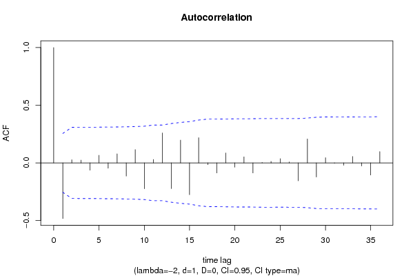
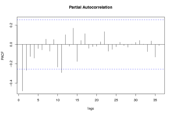
Title produced by software

(Partial) Autocorrelation Function

Date of computation

Fri, 04 Dec 2009 08:17:34 -0700

Cite this page as follows

Statistical Computations at FreeStatistics.org, Office for Research Development and Education, URL https://freestatistics.org/blog/index.php?v=date/2009/Dec/04/t1259939896l8ogerop4iiwje3.htm/, Retrieved Sun, 28 Apr 2024 00:13:57 +0000

Statistical Computations at FreeStatistics.org, Office for Research Development and Education, URL https://freestatistics.org/blog/index.php?pk=63740, Retrieved Sun, 28 Apr 2024 00:13:57 +0000

QR Codes:

Paste this QR Code to cite your computation.

Original text written by user:

IsPrivate?

No (this computation is public)

User-defined keywords

Estimated Impact

131

Family? (F = Feedback message, R = changed R code, M = changed R Module, P = changed Parameters, D = changed Data)

-     [Univariate Explorative Data Analysis] [Run Sequence gebo...] [2008-12-12 13:32:37] [76963dc1903f0f612b6153510a3818cf]
- R  D  [Univariate Explorative Data Analysis] [Run Sequence gebo...] [2008-12-17 12:14:40] [76963dc1903f0f612b6153510a3818cf]
-         [Univariate Explorative Data Analysis] [Run Sequence Plot...] [2008-12-22 18:19:51] [1ce0d16c8f4225c977b42c8fa93bc163]
- RMP       [(Partial) Autocorrelation Function] [Identifying Integ...] [2009-11-22 12:16:10] [b98453cac15ba1066b407e146608df68]
-   PD        [(Partial) Autocorrelation Function] [Ws 8.2] [2009-11-25 19:27:18] [830e13ac5e5ac1e5b21c6af0c149b21d]
-   PD            [(Partial) Autocorrelation Function] [WS 9 ACF] [2009-12-04 15:17:34] [51118f1042b56b16d340924f16263174] [Current]
- RMPD              [Harrell-Davis Quantiles] [Ws 9 Harrel Davis] [2009-12-04 15:59:51] [830e13ac5e5ac1e5b21c6af0c149b21d] 
-   PD              [(Partial) Autocorrelation Function] [ws9 ACF] [2009-12-04 18:53:32] [95cead3ebb75668735f848316249436a] 
-                     [(Partial) Autocorrelation Function] [WS9 ACF] [2009-12-04 19:28:39] [95cead3ebb75668735f848316249436a] 
-   PD              [(Partial) Autocorrelation Function] [ws9 acf] [2009-12-04 20:29:00] [95cead3ebb75668735f848316249436a] 
- R P                 [(Partial) Autocorrelation Function] [] [2009-12-10 16:08:15] [9b30bff5dd5a100f8196daf92e735633] 
-   PD              [(Partial) Autocorrelation Function] [verbetering works...] [2009-12-11 09:51:41] [f1a50df816abcbb519e7637ff6b72fa0] 

Feedback Forum

Post a new message

Dataseries X:

Download CSV

Histogram

Boxplots

100
96,21064363
96,31280765
107,1793443
114,9066592
92,56060184
114,9995356
107,1236185
117,7765394
107,3650971
106,2970187
114,5072908
98,0031578
103,0649206
100,2879168
104,6066685
111,1544534
104,9874617
109,9284852
111,5352466
132,4974459
100,3436426
123,0983561
114,2379493
104,569518
109,0833101
106,9843039
133,6769759
124,8537197
122,5132349
116,8013374
116,0118882
129,7575926
125,1973623
143,7912139
127,9465032
130,2962757
108,4424631
129,3675118
143,6797622
131,8844618
117,6186496
118,9560695
104,8202842
134,624315
140,401226
143,8005015
153,4317823
153,2924677
127,3149438
153,5525216
136,9276493
131,7730101
144,3391845
107,4208229
113,6249652
124,2221603
102,0618557
96,36853348
111,6838488

Summary of computational transaction
Raw Input	view raw input (R code)
Raw Output	view raw output of R engine
Computing time	2 seconds
R Server	'Gwilym Jenkins' @ 72.249.127.135

\begin{tabular}{lllllllll}
\hline
Summary of computational transaction \tabularnewline
Raw Input & view raw input (R code)  \tabularnewline
Raw Output & view raw output of R engine  \tabularnewline
Computing time & 2 seconds \tabularnewline
R Server & 'Gwilym Jenkins' @ 72.249.127.135 \tabularnewline
\hline
\end{tabular}
%Source: https://freestatistics.org/blog/index.php?pk=63740&T=0

[TABLE]
[ROW][C]Summary of computational transaction[/C][/ROW]
[ROW][C]Raw Input[/C][C]view raw input (R code) [/C][/ROW]
[ROW][C]Raw Output[/C][C]view raw output of R engine [/C][/ROW]
[ROW][C]Computing time[/C][C]2 seconds[/C][/ROW]
[ROW][C]R Server[/C][C]'Gwilym Jenkins' @ 72.249.127.135[/C][/ROW]
[/TABLE]
Source: https://freestatistics.org/blog/index.php?pk=63740&T=0

Globally Unique Identifier (entire table): ba.freestatistics.org/blog/index.php?pk=63740&T=0

As an alternative you can also use a QR Code:

The GUIDs for individual cells are displayed in the table below:

Summary of computational transaction
Raw Input	view raw input (R code)
Raw Output	view raw output of R engine
Computing time	2 seconds
R Server	'Gwilym Jenkins' @ 72.249.127.135

Autocorrelation Function
Time lag k	ACF(k)	T-STAT	P-value
1	-0.482267	-3.7044	0.000234
2	0.026608	0.2044	0.41938
3	0.023837	0.1831	0.427676
4	-0.063349	-0.4866	0.314174
5	0.065818	0.5056	0.307525
6	-0.046766	-0.3592	0.360359
7	0.078612	0.6038	0.274137
8	-0.114248	-0.8776	0.191872
9	0.114986	0.8832	0.190349
10	-0.22475	-1.7263	0.04476
11	0.029542	0.2269	0.410636
12	0.259365	1.9922	0.02549
13	-0.222875	-1.7119	0.04608
14	0.19777	1.5191	0.06704
15	-0.275816	-2.1186	0.019173
16	0.218606	1.6791	0.049206
17	-0.015405	-0.1183	0.453105
18	-0.087289	-0.6705	0.252585
19	0.086118	0.6615	0.255439
20	-0.037635	-0.2891	0.386766
21	0.052721	0.405	0.343486
22	-0.08747	-0.6719	0.252144
23	0.003865	0.0297	0.488209
24	0.013075	0.1004	0.460172
25	0.036745	0.2822	0.389373
26	0.008095	0.0622	0.475315
27	-0.155549	-1.1948	0.118474
28	0.207593	1.5946	0.058078
29	-0.122918	-0.9441	0.174472
30	0.045213	0.3473	0.364805
31	-0.002989	-0.023	0.490882
32	-0.020821	-0.1599	0.436741
33	0.055426	0.4257	0.335924
34	-0.02673	-0.2053	0.419015
35	-0.105379	-0.8094	0.21076
36	0.098343	0.7554	0.226511

\begin{tabular}{lllllllll}
\hline
Autocorrelation Function \tabularnewline
Time lag k & ACF(k) & T-STAT & P-value \tabularnewline
1 & -0.482267 & -3.7044 & 0.000234 \tabularnewline
2 & 0.026608 & 0.2044 & 0.41938 \tabularnewline
3 & 0.023837 & 0.1831 & 0.427676 \tabularnewline
4 & -0.063349 & -0.4866 & 0.314174 \tabularnewline
5 & 0.065818 & 0.5056 & 0.307525 \tabularnewline
6 & -0.046766 & -0.3592 & 0.360359 \tabularnewline
7 & 0.078612 & 0.6038 & 0.274137 \tabularnewline
8 & -0.114248 & -0.8776 & 0.191872 \tabularnewline
9 & 0.114986 & 0.8832 & 0.190349 \tabularnewline
10 & -0.22475 & -1.7263 & 0.04476 \tabularnewline
11 & 0.029542 & 0.2269 & 0.410636 \tabularnewline
12 & 0.259365 & 1.9922 & 0.02549 \tabularnewline
13 & -0.222875 & -1.7119 & 0.04608 \tabularnewline
14 & 0.19777 & 1.5191 & 0.06704 \tabularnewline
15 & -0.275816 & -2.1186 & 0.019173 \tabularnewline
16 & 0.218606 & 1.6791 & 0.049206 \tabularnewline
17 & -0.015405 & -0.1183 & 0.453105 \tabularnewline
18 & -0.087289 & -0.6705 & 0.252585 \tabularnewline
19 & 0.086118 & 0.6615 & 0.255439 \tabularnewline
20 & -0.037635 & -0.2891 & 0.386766 \tabularnewline
21 & 0.052721 & 0.405 & 0.343486 \tabularnewline
22 & -0.08747 & -0.6719 & 0.252144 \tabularnewline
23 & 0.003865 & 0.0297 & 0.488209 \tabularnewline
24 & 0.013075 & 0.1004 & 0.460172 \tabularnewline
25 & 0.036745 & 0.2822 & 0.389373 \tabularnewline
26 & 0.008095 & 0.0622 & 0.475315 \tabularnewline
27 & -0.155549 & -1.1948 & 0.118474 \tabularnewline
28 & 0.207593 & 1.5946 & 0.058078 \tabularnewline
29 & -0.122918 & -0.9441 & 0.174472 \tabularnewline
30 & 0.045213 & 0.3473 & 0.364805 \tabularnewline
31 & -0.002989 & -0.023 & 0.490882 \tabularnewline
32 & -0.020821 & -0.1599 & 0.436741 \tabularnewline
33 & 0.055426 & 0.4257 & 0.335924 \tabularnewline
34 & -0.02673 & -0.2053 & 0.419015 \tabularnewline
35 & -0.105379 & -0.8094 & 0.21076 \tabularnewline
36 & 0.098343 & 0.7554 & 0.226511 \tabularnewline
\hline
\end{tabular}
%Source: https://freestatistics.org/blog/index.php?pk=63740&T=1

[TABLE]
[ROW][C]Autocorrelation Function[/C][/ROW]
[ROW][C]Time lag k[/C][C]ACF(k)[/C][C]T-STAT[/C][C]P-value[/C][/ROW]
[ROW][C]1[/C][C]-0.482267[/C][C]-3.7044[/C][C]0.000234[/C][/ROW]
[ROW][C]2[/C][C]0.026608[/C][C]0.2044[/C][C]0.41938[/C][/ROW]
[ROW][C]3[/C][C]0.023837[/C][C]0.1831[/C][C]0.427676[/C][/ROW]
[ROW][C]4[/C][C]-0.063349[/C][C]-0.4866[/C][C]0.314174[/C][/ROW]
[ROW][C]5[/C][C]0.065818[/C][C]0.5056[/C][C]0.307525[/C][/ROW]
[ROW][C]6[/C][C]-0.046766[/C][C]-0.3592[/C][C]0.360359[/C][/ROW]
[ROW][C]7[/C][C]0.078612[/C][C]0.6038[/C][C]0.274137[/C][/ROW]
[ROW][C]8[/C][C]-0.114248[/C][C]-0.8776[/C][C]0.191872[/C][/ROW]
[ROW][C]9[/C][C]0.114986[/C][C]0.8832[/C][C]0.190349[/C][/ROW]
[ROW][C]10[/C][C]-0.22475[/C][C]-1.7263[/C][C]0.04476[/C][/ROW]
[ROW][C]11[/C][C]0.029542[/C][C]0.2269[/C][C]0.410636[/C][/ROW]
[ROW][C]12[/C][C]0.259365[/C][C]1.9922[/C][C]0.02549[/C][/ROW]
[ROW][C]13[/C][C]-0.222875[/C][C]-1.7119[/C][C]0.04608[/C][/ROW]
[ROW][C]14[/C][C]0.19777[/C][C]1.5191[/C][C]0.06704[/C][/ROW]
[ROW][C]15[/C][C]-0.275816[/C][C]-2.1186[/C][C]0.019173[/C][/ROW]
[ROW][C]16[/C][C]0.218606[/C][C]1.6791[/C][C]0.049206[/C][/ROW]
[ROW][C]17[/C][C]-0.015405[/C][C]-0.1183[/C][C]0.453105[/C][/ROW]
[ROW][C]18[/C][C]-0.087289[/C][C]-0.6705[/C][C]0.252585[/C][/ROW]
[ROW][C]19[/C][C]0.086118[/C][C]0.6615[/C][C]0.255439[/C][/ROW]
[ROW][C]20[/C][C]-0.037635[/C][C]-0.2891[/C][C]0.386766[/C][/ROW]
[ROW][C]21[/C][C]0.052721[/C][C]0.405[/C][C]0.343486[/C][/ROW]
[ROW][C]22[/C][C]-0.08747[/C][C]-0.6719[/C][C]0.252144[/C][/ROW]
[ROW][C]23[/C][C]0.003865[/C][C]0.0297[/C][C]0.488209[/C][/ROW]
[ROW][C]24[/C][C]0.013075[/C][C]0.1004[/C][C]0.460172[/C][/ROW]
[ROW][C]25[/C][C]0.036745[/C][C]0.2822[/C][C]0.389373[/C][/ROW]
[ROW][C]26[/C][C]0.008095[/C][C]0.0622[/C][C]0.475315[/C][/ROW]
[ROW][C]27[/C][C]-0.155549[/C][C]-1.1948[/C][C]0.118474[/C][/ROW]
[ROW][C]28[/C][C]0.207593[/C][C]1.5946[/C][C]0.058078[/C][/ROW]
[ROW][C]29[/C][C]-0.122918[/C][C]-0.9441[/C][C]0.174472[/C][/ROW]
[ROW][C]30[/C][C]0.045213[/C][C]0.3473[/C][C]0.364805[/C][/ROW]
[ROW][C]31[/C][C]-0.002989[/C][C]-0.023[/C][C]0.490882[/C][/ROW]
[ROW][C]32[/C][C]-0.020821[/C][C]-0.1599[/C][C]0.436741[/C][/ROW]
[ROW][C]33[/C][C]0.055426[/C][C]0.4257[/C][C]0.335924[/C][/ROW]
[ROW][C]34[/C][C]-0.02673[/C][C]-0.2053[/C][C]0.419015[/C][/ROW]
[ROW][C]35[/C][C]-0.105379[/C][C]-0.8094[/C][C]0.21076[/C][/ROW]
[ROW][C]36[/C][C]0.098343[/C][C]0.7554[/C][C]0.226511[/C][/ROW]
[/TABLE]
Source: https://freestatistics.org/blog/index.php?pk=63740&T=1

Globally Unique Identifier (entire table): ba.freestatistics.org/blog/index.php?pk=63740&T=1

As an alternative you can also use a QR Code:

The GUIDs for individual cells are displayed in the table below:

Autocorrelation Function
Time lag k	ACF(k)	T-STAT	P-value
1	-0.482267	-3.7044	0.000234
2	0.026608	0.2044	0.41938
3	0.023837	0.1831	0.427676
4	-0.063349	-0.4866	0.314174
5	0.065818	0.5056	0.307525
6	-0.046766	-0.3592	0.360359
7	0.078612	0.6038	0.274137
8	-0.114248	-0.8776	0.191872
9	0.114986	0.8832	0.190349
10	-0.22475	-1.7263	0.04476
11	0.029542	0.2269	0.410636
12	0.259365	1.9922	0.02549
13	-0.222875	-1.7119	0.04608
14	0.19777	1.5191	0.06704
15	-0.275816	-2.1186	0.019173
16	0.218606	1.6791	0.049206
17	-0.015405	-0.1183	0.453105
18	-0.087289	-0.6705	0.252585
19	0.086118	0.6615	0.255439
20	-0.037635	-0.2891	0.386766
21	0.052721	0.405	0.343486
22	-0.08747	-0.6719	0.252144
23	0.003865	0.0297	0.488209
24	0.013075	0.1004	0.460172
25	0.036745	0.2822	0.389373
26	0.008095	0.0622	0.475315
27	-0.155549	-1.1948	0.118474
28	0.207593	1.5946	0.058078
29	-0.122918	-0.9441	0.174472
30	0.045213	0.3473	0.364805
31	-0.002989	-0.023	0.490882
32	-0.020821	-0.1599	0.436741
33	0.055426	0.4257	0.335924
34	-0.02673	-0.2053	0.419015
35	-0.105379	-0.8094	0.21076
36	0.098343	0.7554	0.226511

Partial Autocorrelation Function
Time lag k	PACF(k)	T-STAT	P-value
1	-0.482267	-3.7044	0.000234
2	-0.268397	-2.0616	0.02183
3	-0.125434	-0.9635	0.169621
4	-0.141633	-1.0879	0.140531
5	-0.042707	-0.328	0.372021
6	-0.05655	-0.4344	0.332802
7	0.055902	0.4294	0.334602
8	-0.070103	-0.5385	0.296139
9	0.051694	0.3971	0.346374
10	-0.234512	-1.8013	0.038382
11	-0.291713	-2.2407	0.014412
12	0.101704	0.7812	0.218904
13	-0.018376	-0.1412	0.444116
14	0.169063	1.2986	0.099567
15	-0.176576	-1.3563	0.090085
16	0.041884	0.3217	0.374402
17	0.111839	0.8591	0.196894
18	-0.040149	-0.3084	0.379435
19	-0.022327	-0.1715	0.432209
20	-0.019031	-0.1462	0.442138
21	0.02828	0.2172	0.414392
22	0.132709	1.0194	0.156098
23	-0.070409	-0.5408	0.295333
24	-0.051602	-0.3964	0.346635
25	-0.024796	-0.1905	0.4248
26	0.024658	0.1894	0.425214
27	-0.011462	-0.088	0.465071
28	-0.028188	-0.2165	0.414667
29	0.003454	0.0265	0.489461
30	0.02242	0.1722	0.431929
31	0.042335	0.3252	0.373098
32	0.003427	0.0263	0.489545
33	-0.074388	-0.5714	0.284955
34	0.036534	0.2806	0.389989
35	-0.130621	-1.0033	0.159903
36	-0.010494	-0.0806	0.468014

\begin{tabular}{lllllllll}
\hline
Partial Autocorrelation Function \tabularnewline
Time lag k & PACF(k) & T-STAT & P-value \tabularnewline
1 & -0.482267 & -3.7044 & 0.000234 \tabularnewline
2 & -0.268397 & -2.0616 & 0.02183 \tabularnewline
3 & -0.125434 & -0.9635 & 0.169621 \tabularnewline
4 & -0.141633 & -1.0879 & 0.140531 \tabularnewline
5 & -0.042707 & -0.328 & 0.372021 \tabularnewline
6 & -0.05655 & -0.4344 & 0.332802 \tabularnewline
7 & 0.055902 & 0.4294 & 0.334602 \tabularnewline
8 & -0.070103 & -0.5385 & 0.296139 \tabularnewline
9 & 0.051694 & 0.3971 & 0.346374 \tabularnewline
10 & -0.234512 & -1.8013 & 0.038382 \tabularnewline
11 & -0.291713 & -2.2407 & 0.014412 \tabularnewline
12 & 0.101704 & 0.7812 & 0.218904 \tabularnewline
13 & -0.018376 & -0.1412 & 0.444116 \tabularnewline
14 & 0.169063 & 1.2986 & 0.099567 \tabularnewline
15 & -0.176576 & -1.3563 & 0.090085 \tabularnewline
16 & 0.041884 & 0.3217 & 0.374402 \tabularnewline
17 & 0.111839 & 0.8591 & 0.196894 \tabularnewline
18 & -0.040149 & -0.3084 & 0.379435 \tabularnewline
19 & -0.022327 & -0.1715 & 0.432209 \tabularnewline
20 & -0.019031 & -0.1462 & 0.442138 \tabularnewline
21 & 0.02828 & 0.2172 & 0.414392 \tabularnewline
22 & 0.132709 & 1.0194 & 0.156098 \tabularnewline
23 & -0.070409 & -0.5408 & 0.295333 \tabularnewline
24 & -0.051602 & -0.3964 & 0.346635 \tabularnewline
25 & -0.024796 & -0.1905 & 0.4248 \tabularnewline
26 & 0.024658 & 0.1894 & 0.425214 \tabularnewline
27 & -0.011462 & -0.088 & 0.465071 \tabularnewline
28 & -0.028188 & -0.2165 & 0.414667 \tabularnewline
29 & 0.003454 & 0.0265 & 0.489461 \tabularnewline
30 & 0.02242 & 0.1722 & 0.431929 \tabularnewline
31 & 0.042335 & 0.3252 & 0.373098 \tabularnewline
32 & 0.003427 & 0.0263 & 0.489545 \tabularnewline
33 & -0.074388 & -0.5714 & 0.284955 \tabularnewline
34 & 0.036534 & 0.2806 & 0.389989 \tabularnewline
35 & -0.130621 & -1.0033 & 0.159903 \tabularnewline
36 & -0.010494 & -0.0806 & 0.468014 \tabularnewline
\hline
\end{tabular}
%Source: https://freestatistics.org/blog/index.php?pk=63740&T=2

[TABLE]
[ROW][C]Partial Autocorrelation Function[/C][/ROW]
[ROW][C]Time lag k[/C][C]PACF(k)[/C][C]T-STAT[/C][C]P-value[/C][/ROW]
[ROW][C]1[/C][C]-0.482267[/C][C]-3.7044[/C][C]0.000234[/C][/ROW]
[ROW][C]2[/C][C]-0.268397[/C][C]-2.0616[/C][C]0.02183[/C][/ROW]
[ROW][C]3[/C][C]-0.125434[/C][C]-0.9635[/C][C]0.169621[/C][/ROW]
[ROW][C]4[/C][C]-0.141633[/C][C]-1.0879[/C][C]0.140531[/C][/ROW]
[ROW][C]5[/C][C]-0.042707[/C][C]-0.328[/C][C]0.372021[/C][/ROW]
[ROW][C]6[/C][C]-0.05655[/C][C]-0.4344[/C][C]0.332802[/C][/ROW]
[ROW][C]7[/C][C]0.055902[/C][C]0.4294[/C][C]0.334602[/C][/ROW]
[ROW][C]8[/C][C]-0.070103[/C][C]-0.5385[/C][C]0.296139[/C][/ROW]
[ROW][C]9[/C][C]0.051694[/C][C]0.3971[/C][C]0.346374[/C][/ROW]
[ROW][C]10[/C][C]-0.234512[/C][C]-1.8013[/C][C]0.038382[/C][/ROW]
[ROW][C]11[/C][C]-0.291713[/C][C]-2.2407[/C][C]0.014412[/C][/ROW]
[ROW][C]12[/C][C]0.101704[/C][C]0.7812[/C][C]0.218904[/C][/ROW]
[ROW][C]13[/C][C]-0.018376[/C][C]-0.1412[/C][C]0.444116[/C][/ROW]
[ROW][C]14[/C][C]0.169063[/C][C]1.2986[/C][C]0.099567[/C][/ROW]
[ROW][C]15[/C][C]-0.176576[/C][C]-1.3563[/C][C]0.090085[/C][/ROW]
[ROW][C]16[/C][C]0.041884[/C][C]0.3217[/C][C]0.374402[/C][/ROW]
[ROW][C]17[/C][C]0.111839[/C][C]0.8591[/C][C]0.196894[/C][/ROW]
[ROW][C]18[/C][C]-0.040149[/C][C]-0.3084[/C][C]0.379435[/C][/ROW]
[ROW][C]19[/C][C]-0.022327[/C][C]-0.1715[/C][C]0.432209[/C][/ROW]
[ROW][C]20[/C][C]-0.019031[/C][C]-0.1462[/C][C]0.442138[/C][/ROW]
[ROW][C]21[/C][C]0.02828[/C][C]0.2172[/C][C]0.414392[/C][/ROW]
[ROW][C]22[/C][C]0.132709[/C][C]1.0194[/C][C]0.156098[/C][/ROW]
[ROW][C]23[/C][C]-0.070409[/C][C]-0.5408[/C][C]0.295333[/C][/ROW]
[ROW][C]24[/C][C]-0.051602[/C][C]-0.3964[/C][C]0.346635[/C][/ROW]
[ROW][C]25[/C][C]-0.024796[/C][C]-0.1905[/C][C]0.4248[/C][/ROW]
[ROW][C]26[/C][C]0.024658[/C][C]0.1894[/C][C]0.425214[/C][/ROW]
[ROW][C]27[/C][C]-0.011462[/C][C]-0.088[/C][C]0.465071[/C][/ROW]
[ROW][C]28[/C][C]-0.028188[/C][C]-0.2165[/C][C]0.414667[/C][/ROW]
[ROW][C]29[/C][C]0.003454[/C][C]0.0265[/C][C]0.489461[/C][/ROW]
[ROW][C]30[/C][C]0.02242[/C][C]0.1722[/C][C]0.431929[/C][/ROW]
[ROW][C]31[/C][C]0.042335[/C][C]0.3252[/C][C]0.373098[/C][/ROW]
[ROW][C]32[/C][C]0.003427[/C][C]0.0263[/C][C]0.489545[/C][/ROW]
[ROW][C]33[/C][C]-0.074388[/C][C]-0.5714[/C][C]0.284955[/C][/ROW]
[ROW][C]34[/C][C]0.036534[/C][C]0.2806[/C][C]0.389989[/C][/ROW]
[ROW][C]35[/C][C]-0.130621[/C][C]-1.0033[/C][C]0.159903[/C][/ROW]
[ROW][C]36[/C][C]-0.010494[/C][C]-0.0806[/C][C]0.468014[/C][/ROW]
[/TABLE]
Source: https://freestatistics.org/blog/index.php?pk=63740&T=2

Globally Unique Identifier (entire table): ba.freestatistics.org/blog/index.php?pk=63740&T=2

As an alternative you can also use a QR Code:

The GUIDs for individual cells are displayed in the table below:

Partial Autocorrelation Function
Time lag k	PACF(k)	T-STAT	P-value
1	-0.482267	-3.7044	0.000234
2	-0.268397	-2.0616	0.02183
3	-0.125434	-0.9635	0.169621
4	-0.141633	-1.0879	0.140531
5	-0.042707	-0.328	0.372021
6	-0.05655	-0.4344	0.332802
7	0.055902	0.4294	0.334602
8	-0.070103	-0.5385	0.296139
9	0.051694	0.3971	0.346374
10	-0.234512	-1.8013	0.038382
11	-0.291713	-2.2407	0.014412
12	0.101704	0.7812	0.218904
13	-0.018376	-0.1412	0.444116
14	0.169063	1.2986	0.099567
15	-0.176576	-1.3563	0.090085
16	0.041884	0.3217	0.374402
17	0.111839	0.8591	0.196894
18	-0.040149	-0.3084	0.379435
19	-0.022327	-0.1715	0.432209
20	-0.019031	-0.1462	0.442138
21	0.02828	0.2172	0.414392
22	0.132709	1.0194	0.156098
23	-0.070409	-0.5408	0.295333
24	-0.051602	-0.3964	0.346635
25	-0.024796	-0.1905	0.4248
26	0.024658	0.1894	0.425214
27	-0.011462	-0.088	0.465071
28	-0.028188	-0.2165	0.414667
29	0.003454	0.0265	0.489461
30	0.02242	0.1722	0.431929
31	0.042335	0.3252	0.373098
32	0.003427	0.0263	0.489545
33	-0.074388	-0.5714	0.284955
34	0.036534	0.2806	0.389989
35	-0.130621	-1.0033	0.159903
36	-0.010494	-0.0806	0.468014

Figure 1

PNG link

Postscript link

PDF link

Figure 2

PNG link

Postscript link

PDF link

Parameters (Session):

par1 = 36 ; par2 = -2.0 ; par3 = 1 ; par4 = 0 ; par5 = 12 ; par6 = MA ; par7 = 0.95 ;

Parameters (R input):

par1 = 36 ; par2 = -2.0 ; par3 = 1 ; par4 = 0 ; par5 = 12 ; par6 = MA ; par7 = 0.95 ;

R code (references can be found in the software module):

if (par1 == 'Default') {
par1 = 10*log10(length(x))
} else {
par1 <- as.numeric(par1)
}
par2 <- as.numeric(par2)
par3 <- as.numeric(par3)
par4 <- as.numeric(par4)
par5 <- as.numeric(par5)
if (par6 == 'White Noise') par6 <- 'white' else par6 <- 'ma'
par7 <- as.numeric(par7)
if (par2 == 0) {
x <- log(x)
} else {
x <- (x ^ par2 - 1) / par2
}
if (par3 > 0) x <- diff(x,lag=1,difference=par3)
if (par4 > 0) x <- diff(x,lag=par5,difference=par4)
bitmap(file='pic1.png')
racf <- acf(x, par1, main='Autocorrelation', xlab='time lag', ylab='ACF', ci.type=par6, ci=par7, sub=paste('(lambda=',par2,', d=',par3,', D=',par4,', CI=', par7, ', CI type=',par6,')',sep=''))
dev.off()
bitmap(file='pic2.png')
rpacf <- pacf(x,par1,main='Partial Autocorrelation',xlab='lags',ylab='PACF')
dev.off()
(myacf <- c(racf$acf))
(mypacf <- c(rpacf$acf))
lengthx <- length(x)
sqrtn <- sqrt(lengthx)
load(file='createtable')
a<-table.start()
a<-table.row.start(a)
a<-table.element(a,'Autocorrelation Function',4,TRUE)
a<-table.row.end(a)
a<-table.row.start(a)
a<-table.element(a,'Time lag k',header=TRUE)
a<-table.element(a,hyperlink('basics.htm','ACF(k)','click here for more information about the Autocorrelation Function'),header=TRUE)
a<-table.element(a,'T-STAT',header=TRUE)
a<-table.element(a,'P-value',header=TRUE)
a<-table.row.end(a)
for (i in 2:(par1+1)) {
a<-table.row.start(a)
a<-table.element(a,i-1,header=TRUE)
a<-table.element(a,round(myacf[i],6))
mytstat <- myacf[i]*sqrtn
a<-table.element(a,round(mytstat,4))
a<-table.element(a,round(1-pt(abs(mytstat),lengthx),6))
a<-table.row.end(a)
}
a<-table.end(a)
table.save(a,file='mytable.tab')
a<-table.start()
a<-table.row.start(a)
a<-table.element(a,'Partial Autocorrelation Function',4,TRUE)
a<-table.row.end(a)
a<-table.row.start(a)
a<-table.element(a,'Time lag k',header=TRUE)
a<-table.element(a,hyperlink('basics.htm','PACF(k)','click here for more information about the Partial Autocorrelation Function'),header=TRUE)
a<-table.element(a,'T-STAT',header=TRUE)
a<-table.element(a,'P-value',header=TRUE)
a<-table.row.end(a)
for (i in 1:par1) {
a<-table.row.start(a)
a<-table.element(a,i,header=TRUE)
a<-table.element(a,round(mypacf[i],6))
mytstat <- mypacf[i]*sqrtn
a<-table.element(a,round(mytstat,4))
a<-table.element(a,round(1-pt(abs(mytstat),lengthx),6))
a<-table.row.end(a)
}
a<-table.end(a)
table.save(a,file='mytable1.tab')

Free Statistics

Description of Statistical Computation

Tree of Dependent Computations

Dataset

Tables (Output of Computation)

Figures (Output of Computation)

Input Parameters & R Code