Repository of Reproducible Computations

Free Statistics

of Irreproducible Research!

Author's title

Author

*The author of this computation has been verified*

R Software Module

rwasp_autocorrelation.wasp

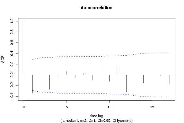
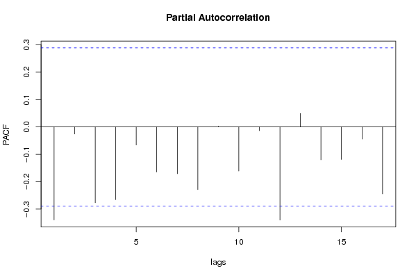
Title produced by software

(Partial) Autocorrelation Function

Date of computation

Fri, 04 Dec 2009 10:22:31 -0700

Cite this page as follows

Statistical Computations at FreeStatistics.org, Office for Research Development and Education, URL https://freestatistics.org/blog/index.php?v=date/2009/Dec/04/t1259947406bv4e4by6opb7ciy.htm/, Retrieved Sat, 27 Apr 2024 20:25:09 +0000

Statistical Computations at FreeStatistics.org, Office for Research Development and Education, URL https://freestatistics.org/blog/index.php?pk=63935, Retrieved Sat, 27 Apr 2024 20:25:09 +0000

QR Codes:

Paste this QR Code to cite your computation.

Original text written by user:

IsPrivate?

No (this computation is public)

User-defined keywords

Estimated Impact

Family? (F = Feedback message, R = changed R code, M = changed R Module, P = changed Parameters, D = changed Data)

-     [Univariate Explorative Data Analysis] [Run Sequence gebo...] [2008-12-12 13:32:37] [76963dc1903f0f612b6153510a3818cf]
- R  D  [Univariate Explorative Data Analysis] [Run Sequence gebo...] [2008-12-17 12:14:40] [76963dc1903f0f612b6153510a3818cf]
-         [Univariate Explorative Data Analysis] [Run Sequence Plot...] [2008-12-22 18:19:51] [1ce0d16c8f4225c977b42c8fa93bc163]
- RMP       [(Partial) Autocorrelation Function] [Identifying Integ...] [2009-11-22 12:26:39] [b98453cac15ba1066b407e146608df68]
-   PD        [(Partial) Autocorrelation Function] [] [2009-11-27 19:38:56] [897115520fe7b6114489bc0eeed64548]
-   P             [(Partial) Autocorrelation Function] [] [2009-12-04 17:22:31] [90c9838c596c9c0a7d0d4c412ffe5b98] [Current]

Feedback Forum

Post a new message

Dataseries X:

Download CSV

Histogram

Boxplots

Summary of computational transaction
Raw Input	view raw input (R code)
Raw Output	view raw output of R engine
Computing time	1 seconds
R Server	'Gwilym Jenkins' @ 72.249.127.135

\begin{tabular}{lllllllll}
\hline
Summary of computational transaction \tabularnewline
Raw Input & view raw input (R code)  \tabularnewline
Raw Output & view raw output of R engine  \tabularnewline
Computing time & 1 seconds \tabularnewline
R Server & 'Gwilym Jenkins' @ 72.249.127.135 \tabularnewline
\hline
\end{tabular}
%Source: https://freestatistics.org/blog/index.php?pk=63935&T=0

[TABLE]
[ROW][C]Summary of computational transaction[/C][/ROW]
[ROW][C]Raw Input[/C][C]view raw input (R code) [/C][/ROW]
[ROW][C]Raw Output[/C][C]view raw output of R engine [/C][/ROW]
[ROW][C]Computing time[/C][C]1 seconds[/C][/ROW]
[ROW][C]R Server[/C][C]'Gwilym Jenkins' @ 72.249.127.135[/C][/ROW]
[/TABLE]
Source: https://freestatistics.org/blog/index.php?pk=63935&T=0

Globally Unique Identifier (entire table): ba.freestatistics.org/blog/index.php?pk=63935&T=0

As an alternative you can also use a QR Code:

The GUIDs for individual cells are displayed in the table below:

Summary of computational transaction
Raw Input	view raw input (R code)
Raw Output	view raw output of R engine
Computing time	1 seconds
R Server	'Gwilym Jenkins' @ 72.249.127.135

Autocorrelation Function
Time lag k	ACF(k)	T-STAT	P-value
1	-0.339712	-2.304	0.012894
2	0.092733	0.6289	0.266247
3	-0.268807	-1.8231	0.037393
4	-0.038382	-0.2603	0.397889
5	0.063851	0.4331	0.333499
6	-0.048361	-0.328	0.372199
7	0.029187	0.198	0.421975
8	-0.098286	-0.6666	0.254177
9	0.183166	1.2423	0.110212
10	-0.120333	-0.8161	0.209314
11	0.160855	1.091	0.140483
12	-0.314107	-2.1304	0.01926
13	0.298785	2.0265	0.024269
14	-0.154157	-1.0455	0.150618
15	0.107788	0.7311	0.234226
16	-0.019235	-0.1305	0.448386
17	-0.17379	-1.1787	0.12229

\begin{tabular}{lllllllll}
\hline
Autocorrelation Function \tabularnewline
Time lag k & ACF(k) & T-STAT & P-value \tabularnewline
1 & -0.339712 & -2.304 & 0.012894 \tabularnewline
2 & 0.092733 & 0.6289 & 0.266247 \tabularnewline
3 & -0.268807 & -1.8231 & 0.037393 \tabularnewline
4 & -0.038382 & -0.2603 & 0.397889 \tabularnewline
5 & 0.063851 & 0.4331 & 0.333499 \tabularnewline
6 & -0.048361 & -0.328 & 0.372199 \tabularnewline
7 & 0.029187 & 0.198 & 0.421975 \tabularnewline
8 & -0.098286 & -0.6666 & 0.254177 \tabularnewline
9 & 0.183166 & 1.2423 & 0.110212 \tabularnewline
10 & -0.120333 & -0.8161 & 0.209314 \tabularnewline
11 & 0.160855 & 1.091 & 0.140483 \tabularnewline
12 & -0.314107 & -2.1304 & 0.01926 \tabularnewline
13 & 0.298785 & 2.0265 & 0.024269 \tabularnewline
14 & -0.154157 & -1.0455 & 0.150618 \tabularnewline
15 & 0.107788 & 0.7311 & 0.234226 \tabularnewline
16 & -0.019235 & -0.1305 & 0.448386 \tabularnewline
17 & -0.17379 & -1.1787 & 0.12229 \tabularnewline
\hline
\end{tabular}
%Source: https://freestatistics.org/blog/index.php?pk=63935&T=1

[TABLE]
[ROW][C]Autocorrelation Function[/C][/ROW]
[ROW][C]Time lag k[/C][C]ACF(k)[/C][C]T-STAT[/C][C]P-value[/C][/ROW]
[ROW][C]1[/C][C]-0.339712[/C][C]-2.304[/C][C]0.012894[/C][/ROW]
[ROW][C]2[/C][C]0.092733[/C][C]0.6289[/C][C]0.266247[/C][/ROW]
[ROW][C]3[/C][C]-0.268807[/C][C]-1.8231[/C][C]0.037393[/C][/ROW]
[ROW][C]4[/C][C]-0.038382[/C][C]-0.2603[/C][C]0.397889[/C][/ROW]
[ROW][C]5[/C][C]0.063851[/C][C]0.4331[/C][C]0.333499[/C][/ROW]
[ROW][C]6[/C][C]-0.048361[/C][C]-0.328[/C][C]0.372199[/C][/ROW]
[ROW][C]7[/C][C]0.029187[/C][C]0.198[/C][C]0.421975[/C][/ROW]
[ROW][C]8[/C][C]-0.098286[/C][C]-0.6666[/C][C]0.254177[/C][/ROW]
[ROW][C]9[/C][C]0.183166[/C][C]1.2423[/C][C]0.110212[/C][/ROW]
[ROW][C]10[/C][C]-0.120333[/C][C]-0.8161[/C][C]0.209314[/C][/ROW]
[ROW][C]11[/C][C]0.160855[/C][C]1.091[/C][C]0.140483[/C][/ROW]
[ROW][C]12[/C][C]-0.314107[/C][C]-2.1304[/C][C]0.01926[/C][/ROW]
[ROW][C]13[/C][C]0.298785[/C][C]2.0265[/C][C]0.024269[/C][/ROW]
[ROW][C]14[/C][C]-0.154157[/C][C]-1.0455[/C][C]0.150618[/C][/ROW]
[ROW][C]15[/C][C]0.107788[/C][C]0.7311[/C][C]0.234226[/C][/ROW]
[ROW][C]16[/C][C]-0.019235[/C][C]-0.1305[/C][C]0.448386[/C][/ROW]
[ROW][C]17[/C][C]-0.17379[/C][C]-1.1787[/C][C]0.12229[/C][/ROW]
[/TABLE]
Source: https://freestatistics.org/blog/index.php?pk=63935&T=1

Globally Unique Identifier (entire table): ba.freestatistics.org/blog/index.php?pk=63935&T=1

As an alternative you can also use a QR Code:

The GUIDs for individual cells are displayed in the table below:

Autocorrelation Function
Time lag k	ACF(k)	T-STAT	P-value
1	-0.339712	-2.304	0.012894
2	0.092733	0.6289	0.266247
3	-0.268807	-1.8231	0.037393
4	-0.038382	-0.2603	0.397889
5	0.063851	0.4331	0.333499
6	-0.048361	-0.328	0.372199
7	0.029187	0.198	0.421975
8	-0.098286	-0.6666	0.254177
9	0.183166	1.2423	0.110212
10	-0.120333	-0.8161	0.209314
11	0.160855	1.091	0.140483
12	-0.314107	-2.1304	0.01926
13	0.298785	2.0265	0.024269
14	-0.154157	-1.0455	0.150618
15	0.107788	0.7311	0.234226
16	-0.019235	-0.1305	0.448386
17	-0.17379	-1.1787	0.12229

Partial Autocorrelation Function
Time lag k	PACF(k)	T-STAT	P-value
1	-0.339712	-2.304	0.012894
2	-0.025629	-0.1738	0.431383
3	-0.277374	-1.8812	0.033138
4	-0.265734	-1.8023	0.039027
5	-0.065951	-0.4473	0.328379
6	-0.164953	-1.1188	0.134524
7	-0.170938	-1.1594	0.126146
8	-0.228854	-1.5522	0.063738
9	0.003023	0.0205	0.491865
10	-0.160883	-1.0912	0.140443
11	-0.01368	-0.0928	0.463239
12	-0.340333	-2.3083	0.012766
13	0.04965	0.3367	0.368921
14	-0.119951	-0.8136	0.210047
15	-0.118755	-0.8054	0.212355
16	-0.044025	-0.2986	0.383297
17	-0.244428	-1.6578	0.052083

\begin{tabular}{lllllllll}
\hline
Partial Autocorrelation Function \tabularnewline
Time lag k & PACF(k) & T-STAT & P-value \tabularnewline
1 & -0.339712 & -2.304 & 0.012894 \tabularnewline
2 & -0.025629 & -0.1738 & 0.431383 \tabularnewline
3 & -0.277374 & -1.8812 & 0.033138 \tabularnewline
4 & -0.265734 & -1.8023 & 0.039027 \tabularnewline
5 & -0.065951 & -0.4473 & 0.328379 \tabularnewline
6 & -0.164953 & -1.1188 & 0.134524 \tabularnewline
7 & -0.170938 & -1.1594 & 0.126146 \tabularnewline
8 & -0.228854 & -1.5522 & 0.063738 \tabularnewline
9 & 0.003023 & 0.0205 & 0.491865 \tabularnewline
10 & -0.160883 & -1.0912 & 0.140443 \tabularnewline
11 & -0.01368 & -0.0928 & 0.463239 \tabularnewline
12 & -0.340333 & -2.3083 & 0.012766 \tabularnewline
13 & 0.04965 & 0.3367 & 0.368921 \tabularnewline
14 & -0.119951 & -0.8136 & 0.210047 \tabularnewline
15 & -0.118755 & -0.8054 & 0.212355 \tabularnewline
16 & -0.044025 & -0.2986 & 0.383297 \tabularnewline
17 & -0.244428 & -1.6578 & 0.052083 \tabularnewline
\hline
\end{tabular}
%Source: https://freestatistics.org/blog/index.php?pk=63935&T=2

[TABLE]
[ROW][C]Partial Autocorrelation Function[/C][/ROW]
[ROW][C]Time lag k[/C][C]PACF(k)[/C][C]T-STAT[/C][C]P-value[/C][/ROW]
[ROW][C]1[/C][C]-0.339712[/C][C]-2.304[/C][C]0.012894[/C][/ROW]
[ROW][C]2[/C][C]-0.025629[/C][C]-0.1738[/C][C]0.431383[/C][/ROW]
[ROW][C]3[/C][C]-0.277374[/C][C]-1.8812[/C][C]0.033138[/C][/ROW]
[ROW][C]4[/C][C]-0.265734[/C][C]-1.8023[/C][C]0.039027[/C][/ROW]
[ROW][C]5[/C][C]-0.065951[/C][C]-0.4473[/C][C]0.328379[/C][/ROW]
[ROW][C]6[/C][C]-0.164953[/C][C]-1.1188[/C][C]0.134524[/C][/ROW]
[ROW][C]7[/C][C]-0.170938[/C][C]-1.1594[/C][C]0.126146[/C][/ROW]
[ROW][C]8[/C][C]-0.228854[/C][C]-1.5522[/C][C]0.063738[/C][/ROW]
[ROW][C]9[/C][C]0.003023[/C][C]0.0205[/C][C]0.491865[/C][/ROW]
[ROW][C]10[/C][C]-0.160883[/C][C]-1.0912[/C][C]0.140443[/C][/ROW]
[ROW][C]11[/C][C]-0.01368[/C][C]-0.0928[/C][C]0.463239[/C][/ROW]
[ROW][C]12[/C][C]-0.340333[/C][C]-2.3083[/C][C]0.012766[/C][/ROW]
[ROW][C]13[/C][C]0.04965[/C][C]0.3367[/C][C]0.368921[/C][/ROW]
[ROW][C]14[/C][C]-0.119951[/C][C]-0.8136[/C][C]0.210047[/C][/ROW]
[ROW][C]15[/C][C]-0.118755[/C][C]-0.8054[/C][C]0.212355[/C][/ROW]
[ROW][C]16[/C][C]-0.044025[/C][C]-0.2986[/C][C]0.383297[/C][/ROW]
[ROW][C]17[/C][C]-0.244428[/C][C]-1.6578[/C][C]0.052083[/C][/ROW]
[/TABLE]
Source: https://freestatistics.org/blog/index.php?pk=63935&T=2

Globally Unique Identifier (entire table): ba.freestatistics.org/blog/index.php?pk=63935&T=2

As an alternative you can also use a QR Code:

The GUIDs for individual cells are displayed in the table below:

Partial Autocorrelation Function
Time lag k	PACF(k)	T-STAT	P-value
1	-0.339712	-2.304	0.012894
2	-0.025629	-0.1738	0.431383
3	-0.277374	-1.8812	0.033138
4	-0.265734	-1.8023	0.039027
5	-0.065951	-0.4473	0.328379
6	-0.164953	-1.1188	0.134524
7	-0.170938	-1.1594	0.126146
8	-0.228854	-1.5522	0.063738
9	0.003023	0.0205	0.491865
10	-0.160883	-1.0912	0.140443
11	-0.01368	-0.0928	0.463239
12	-0.340333	-2.3083	0.012766
13	0.04965	0.3367	0.368921
14	-0.119951	-0.8136	0.210047
15	-0.118755	-0.8054	0.212355
16	-0.044025	-0.2986	0.383297
17	-0.244428	-1.6578	0.052083

Figure 1

PNG link

Postscript link

PDF link

Figure 2

PNG link

Postscript link

PDF link

Parameters (Session):

par1 = Default ; par2 = 1 ; par3 = 2 ; par4 = 1 ; par5 = 12 ; par6 = MA ; par7 = 0.95 ;

Parameters (R input):

par1 = Default ; par2 = 1 ; par3 = 2 ; par4 = 1 ; par5 = 12 ; par6 = MA ; par7 = 0.95 ;

R code (references can be found in the software module):

if (par1 == 'Default') {
par1 = 10*log10(length(x))
} else {
par1 <- as.numeric(par1)
}
par2 <- as.numeric(par2)
par3 <- as.numeric(par3)
par4 <- as.numeric(par4)
par5 <- as.numeric(par5)
if (par6 == 'White Noise') par6 <- 'white' else par6 <- 'ma'
par7 <- as.numeric(par7)
if (par2 == 0) {
x <- log(x)
} else {
x <- (x ^ par2 - 1) / par2
}
if (par3 > 0) x <- diff(x,lag=1,difference=par3)
if (par4 > 0) x <- diff(x,lag=par5,difference=par4)
bitmap(file='pic1.png')
racf <- acf(x, par1, main='Autocorrelation', xlab='time lag', ylab='ACF', ci.type=par6, ci=par7, sub=paste('(lambda=',par2,', d=',par3,', D=',par4,', CI=', par7, ', CI type=',par6,')',sep=''))
dev.off()
bitmap(file='pic2.png')
rpacf <- pacf(x,par1,main='Partial Autocorrelation',xlab='lags',ylab='PACF')
dev.off()
(myacf <- c(racf$acf))
(mypacf <- c(rpacf$acf))
lengthx <- length(x)
sqrtn <- sqrt(lengthx)
load(file='createtable')
a<-table.start()
a<-table.row.start(a)
a<-table.element(a,'Autocorrelation Function',4,TRUE)
a<-table.row.end(a)
a<-table.row.start(a)
a<-table.element(a,'Time lag k',header=TRUE)
a<-table.element(a,hyperlink('basics.htm','ACF(k)','click here for more information about the Autocorrelation Function'),header=TRUE)
a<-table.element(a,'T-STAT',header=TRUE)
a<-table.element(a,'P-value',header=TRUE)
a<-table.row.end(a)
for (i in 2:(par1+1)) {
a<-table.row.start(a)
a<-table.element(a,i-1,header=TRUE)
a<-table.element(a,round(myacf[i],6))
mytstat <- myacf[i]*sqrtn
a<-table.element(a,round(mytstat,4))
a<-table.element(a,round(1-pt(abs(mytstat),lengthx),6))
a<-table.row.end(a)
}
a<-table.end(a)
table.save(a,file='mytable.tab')
a<-table.start()
a<-table.row.start(a)
a<-table.element(a,'Partial Autocorrelation Function',4,TRUE)
a<-table.row.end(a)
a<-table.row.start(a)
a<-table.element(a,'Time lag k',header=TRUE)
a<-table.element(a,hyperlink('basics.htm','PACF(k)','click here for more information about the Partial Autocorrelation Function'),header=TRUE)
a<-table.element(a,'T-STAT',header=TRUE)
a<-table.element(a,'P-value',header=TRUE)
a<-table.row.end(a)
for (i in 1:par1) {
a<-table.row.start(a)
a<-table.element(a,i,header=TRUE)
a<-table.element(a,round(mypacf[i],6))
mytstat <- mypacf[i]*sqrtn
a<-table.element(a,round(mytstat,4))
a<-table.element(a,round(1-pt(abs(mytstat),lengthx),6))
a<-table.row.end(a)
}
a<-table.end(a)
table.save(a,file='mytable1.tab')

Free Statistics

Description of Statistical Computation

Tree of Dependent Computations

Dataset

Tables (Output of Computation)

Figures (Output of Computation)

Input Parameters & R Code