Repository of Reproducible Computations

Free Statistics

of Irreproducible Research!

Author's title

Author

*The author of this computation has been verified*

R Software Module

rwasp_autocorrelation.wasp

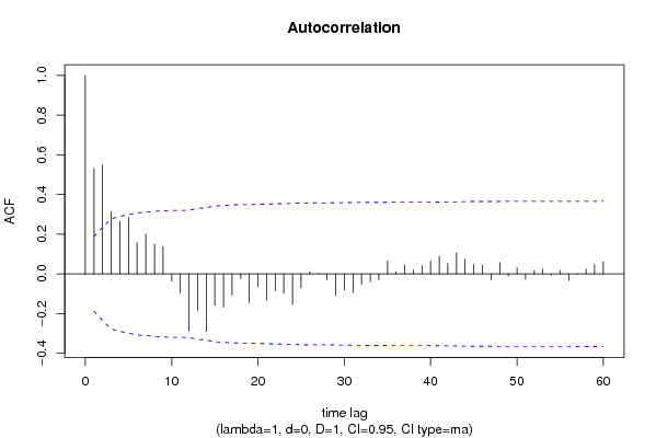
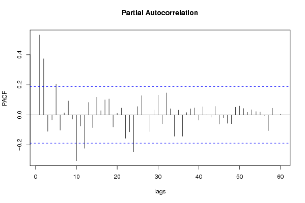
Title produced by software

(Partial) Autocorrelation Function

Date of computation

Wed, 09 Dec 2009 12:28:23 -0700

Cite this page as follows

Statistical Computations at FreeStatistics.org, Office for Research Development and Education, URL https://freestatistics.org/blog/index.php?v=date/2009/Dec/09/t12603870444et77r6rs3uhvsf.htm/, Retrieved Mon, 29 Apr 2024 14:32:10 +0000

Statistical Computations at FreeStatistics.org, Office for Research Development and Education, URL https://freestatistics.org/blog/index.php?pk=65170, Retrieved Mon, 29 Apr 2024 14:32:10 +0000

QR Codes:

Paste this QR Code to cite your computation.

Original text written by user:

IsPrivate?

No (this computation is public)

User-defined keywords

ShwWs9 verbetering

Estimated Impact

122

Family? (F = Feedback message, R = changed R code, M = changed R Module, P = changed Parameters, D = changed Data)

-     [Univariate Explorative Data Analysis] [Run Sequence gebo...] [2008-12-12 13:32:37] [76963dc1903f0f612b6153510a3818cf]
- R  D  [Univariate Explorative Data Analysis] [Run Sequence gebo...] [2008-12-17 12:14:40] [76963dc1903f0f612b6153510a3818cf]
-         [Univariate Explorative Data Analysis] [Run Sequence Plot...] [2008-12-22 18:19:51] [1ce0d16c8f4225c977b42c8fa93bc163]
- RMP       [(Partial) Autocorrelation Function] [Identifying Integ...] [2009-11-22 12:16:10] [b98453cac15ba1066b407e146608df68]
- R PD        [(Partial) Autocorrelation Function] [WS08 - PACF d = 1...] [2009-11-25 20:49:28] [df6326eec97a6ca984a853b142930499]
-   P             [(Partial) Autocorrelation Function] [Verbetering Works...] [2009-12-09 19:28:23] [51108381f3361ca8af49c4f74052c840] [Current]

Feedback Forum

Post a new message

Dataseries X:

Download CSV

Histogram

Boxplots

Summary of computational transaction
Raw Input	view raw input (R code)
Raw Output	view raw output of R engine
Computing time	2 seconds
R Server	'Gwilym Jenkins' @ 72.249.127.135

\begin{tabular}{lllllllll}
\hline
Summary of computational transaction \tabularnewline
Raw Input & view raw input (R code)  \tabularnewline
Raw Output & view raw output of R engine  \tabularnewline
Computing time & 2 seconds \tabularnewline
R Server & 'Gwilym Jenkins' @ 72.249.127.135 \tabularnewline
\hline
\end{tabular}
%Source: https://freestatistics.org/blog/index.php?pk=65170&T=0

[TABLE]
[ROW][C]Summary of computational transaction[/C][/ROW]
[ROW][C]Raw Input[/C][C]view raw input (R code) [/C][/ROW]
[ROW][C]Raw Output[/C][C]view raw output of R engine [/C][/ROW]
[ROW][C]Computing time[/C][C]2 seconds[/C][/ROW]
[ROW][C]R Server[/C][C]'Gwilym Jenkins' @ 72.249.127.135[/C][/ROW]
[/TABLE]
Source: https://freestatistics.org/blog/index.php?pk=65170&T=0

Globally Unique Identifier (entire table): ba.freestatistics.org/blog/index.php?pk=65170&T=0

As an alternative you can also use a QR Code:

The GUIDs for individual cells are displayed in the table below:

Summary of computational transaction
Raw Input	view raw input (R code)
Raw Output	view raw output of R engine
Computing time	2 seconds
R Server	'Gwilym Jenkins' @ 72.249.127.135

Autocorrelation Function
Time lag k	ACF(k)	T-STAT	P-value
1	0.531042	5.5188	0
2	0.549794	5.7136	0
3	0.3133	3.2559	0.000755
4	0.263964	2.7432	0.003563
5	0.284798	2.9597	0.001893
6	0.156377	1.6251	0.053526
7	0.199438	2.0726	0.020294
8	0.149113	1.5496	0.062078
9	0.137391	1.4278	0.078116
10	-0.036796	-0.3824	0.351459
11	-0.095297	-0.9904	0.162108
12	-0.28843	-2.9974	0.001689
13	-0.182828	-1.9	0.03005
14	-0.289845	-3.0122	0.001616
15	-0.158137	-1.6434	0.051604
16	-0.167499	-1.7407	0.042292
17	-0.106471	-1.1065	0.13549
18	-0.024721	-0.2569	0.398871
19	-0.144899	-1.5058	0.067515
20	-0.064273	-0.6679	0.252797
21	-0.133646	-1.3889	0.083862
22	-0.086261	-0.8964	0.186003
23	-0.098533	-1.024	0.154066
24	-0.154306	-1.6036	0.055862
25	-0.068971	-0.7168	0.237531
26	0.011319	0.1176	0.453288
27	0.002835	0.0295	0.488274
28	-0.030544	-0.3174	0.375768
29	-0.10714	-1.1134	0.133997
30	-0.080028	-0.8317	0.203714
31	-0.092823	-0.9646	0.168438
32	-0.051547	-0.5357	0.296637
33	-0.039625	-0.4118	0.340654
34	-0.029239	-0.3039	0.380909
35	0.063661	0.6616	0.254823
36	0.011671	0.1213	0.451842
37	0.045695	0.4749	0.317918
38	0.020175	0.2097	0.417163
39	0.04007	0.4164	0.338966
40	0.064915	0.6746	0.250679
41	0.08856	0.9203	0.179722
42	0.052534	0.5459	0.293113
43	0.106768	1.1096	0.134826
44	0.073958	0.7686	0.221907
45	0.046724	0.4856	0.314128
46	0.045457	0.4724	0.318796
47	-0.02967	-0.3083	0.379207
48	0.056998	0.5923	0.277432
49	-0.010502	-0.1091	0.456649
50	0.030208	0.3139	0.377091
51	-0.025661	-0.2667	0.395112
52	0.017258	0.1793	0.429001
53	0.023555	0.2448	0.403541
54	-0.00738	-0.0767	0.469502
55	0.017823	0.1852	0.426701
56	-0.033292	-0.346	0.365017
57	-0.00336	-0.0349	0.486105
58	0.02396	0.249	0.401919
59	0.045571	0.4736	0.318374
60	0.062074	0.6451	0.260119

\begin{tabular}{lllllllll}
\hline
Autocorrelation Function \tabularnewline
Time lag k & ACF(k) & T-STAT & P-value \tabularnewline
1 & 0.531042 & 5.5188 & 0 \tabularnewline
2 & 0.549794 & 5.7136 & 0 \tabularnewline
3 & 0.3133 & 3.2559 & 0.000755 \tabularnewline
4 & 0.263964 & 2.7432 & 0.003563 \tabularnewline
5 & 0.284798 & 2.9597 & 0.001893 \tabularnewline
6 & 0.156377 & 1.6251 & 0.053526 \tabularnewline
7 & 0.199438 & 2.0726 & 0.020294 \tabularnewline
8 & 0.149113 & 1.5496 & 0.062078 \tabularnewline
9 & 0.137391 & 1.4278 & 0.078116 \tabularnewline
10 & -0.036796 & -0.3824 & 0.351459 \tabularnewline
11 & -0.095297 & -0.9904 & 0.162108 \tabularnewline
12 & -0.28843 & -2.9974 & 0.001689 \tabularnewline
13 & -0.182828 & -1.9 & 0.03005 \tabularnewline
14 & -0.289845 & -3.0122 & 0.001616 \tabularnewline
15 & -0.158137 & -1.6434 & 0.051604 \tabularnewline
16 & -0.167499 & -1.7407 & 0.042292 \tabularnewline
17 & -0.106471 & -1.1065 & 0.13549 \tabularnewline
18 & -0.024721 & -0.2569 & 0.398871 \tabularnewline
19 & -0.144899 & -1.5058 & 0.067515 \tabularnewline
20 & -0.064273 & -0.6679 & 0.252797 \tabularnewline
21 & -0.133646 & -1.3889 & 0.083862 \tabularnewline
22 & -0.086261 & -0.8964 & 0.186003 \tabularnewline
23 & -0.098533 & -1.024 & 0.154066 \tabularnewline
24 & -0.154306 & -1.6036 & 0.055862 \tabularnewline
25 & -0.068971 & -0.7168 & 0.237531 \tabularnewline
26 & 0.011319 & 0.1176 & 0.453288 \tabularnewline
27 & 0.002835 & 0.0295 & 0.488274 \tabularnewline
28 & -0.030544 & -0.3174 & 0.375768 \tabularnewline
29 & -0.10714 & -1.1134 & 0.133997 \tabularnewline
30 & -0.080028 & -0.8317 & 0.203714 \tabularnewline
31 & -0.092823 & -0.9646 & 0.168438 \tabularnewline
32 & -0.051547 & -0.5357 & 0.296637 \tabularnewline
33 & -0.039625 & -0.4118 & 0.340654 \tabularnewline
34 & -0.029239 & -0.3039 & 0.380909 \tabularnewline
35 & 0.063661 & 0.6616 & 0.254823 \tabularnewline
36 & 0.011671 & 0.1213 & 0.451842 \tabularnewline
37 & 0.045695 & 0.4749 & 0.317918 \tabularnewline
38 & 0.020175 & 0.2097 & 0.417163 \tabularnewline
39 & 0.04007 & 0.4164 & 0.338966 \tabularnewline
40 & 0.064915 & 0.6746 & 0.250679 \tabularnewline
41 & 0.08856 & 0.9203 & 0.179722 \tabularnewline
42 & 0.052534 & 0.5459 & 0.293113 \tabularnewline
43 & 0.106768 & 1.1096 & 0.134826 \tabularnewline
44 & 0.073958 & 0.7686 & 0.221907 \tabularnewline
45 & 0.046724 & 0.4856 & 0.314128 \tabularnewline
46 & 0.045457 & 0.4724 & 0.318796 \tabularnewline
47 & -0.02967 & -0.3083 & 0.379207 \tabularnewline
48 & 0.056998 & 0.5923 & 0.277432 \tabularnewline
49 & -0.010502 & -0.1091 & 0.456649 \tabularnewline
50 & 0.030208 & 0.3139 & 0.377091 \tabularnewline
51 & -0.025661 & -0.2667 & 0.395112 \tabularnewline
52 & 0.017258 & 0.1793 & 0.429001 \tabularnewline
53 & 0.023555 & 0.2448 & 0.403541 \tabularnewline
54 & -0.00738 & -0.0767 & 0.469502 \tabularnewline
55 & 0.017823 & 0.1852 & 0.426701 \tabularnewline
56 & -0.033292 & -0.346 & 0.365017 \tabularnewline
57 & -0.00336 & -0.0349 & 0.486105 \tabularnewline
58 & 0.02396 & 0.249 & 0.401919 \tabularnewline
59 & 0.045571 & 0.4736 & 0.318374 \tabularnewline
60 & 0.062074 & 0.6451 & 0.260119 \tabularnewline
\hline
\end{tabular}
%Source: https://freestatistics.org/blog/index.php?pk=65170&T=1

[TABLE]
[ROW][C]Autocorrelation Function[/C][/ROW]
[ROW][C]Time lag k[/C][C]ACF(k)[/C][C]T-STAT[/C][C]P-value[/C][/ROW]
[ROW][C]1[/C][C]0.531042[/C][C]5.5188[/C][C]0[/C][/ROW]
[ROW][C]2[/C][C]0.549794[/C][C]5.7136[/C][C]0[/C][/ROW]
[ROW][C]3[/C][C]0.3133[/C][C]3.2559[/C][C]0.000755[/C][/ROW]
[ROW][C]4[/C][C]0.263964[/C][C]2.7432[/C][C]0.003563[/C][/ROW]
[ROW][C]5[/C][C]0.284798[/C][C]2.9597[/C][C]0.001893[/C][/ROW]
[ROW][C]6[/C][C]0.156377[/C][C]1.6251[/C][C]0.053526[/C][/ROW]
[ROW][C]7[/C][C]0.199438[/C][C]2.0726[/C][C]0.020294[/C][/ROW]
[ROW][C]8[/C][C]0.149113[/C][C]1.5496[/C][C]0.062078[/C][/ROW]
[ROW][C]9[/C][C]0.137391[/C][C]1.4278[/C][C]0.078116[/C][/ROW]
[ROW][C]10[/C][C]-0.036796[/C][C]-0.3824[/C][C]0.351459[/C][/ROW]
[ROW][C]11[/C][C]-0.095297[/C][C]-0.9904[/C][C]0.162108[/C][/ROW]
[ROW][C]12[/C][C]-0.28843[/C][C]-2.9974[/C][C]0.001689[/C][/ROW]
[ROW][C]13[/C][C]-0.182828[/C][C]-1.9[/C][C]0.03005[/C][/ROW]
[ROW][C]14[/C][C]-0.289845[/C][C]-3.0122[/C][C]0.001616[/C][/ROW]
[ROW][C]15[/C][C]-0.158137[/C][C]-1.6434[/C][C]0.051604[/C][/ROW]
[ROW][C]16[/C][C]-0.167499[/C][C]-1.7407[/C][C]0.042292[/C][/ROW]
[ROW][C]17[/C][C]-0.106471[/C][C]-1.1065[/C][C]0.13549[/C][/ROW]
[ROW][C]18[/C][C]-0.024721[/C][C]-0.2569[/C][C]0.398871[/C][/ROW]
[ROW][C]19[/C][C]-0.144899[/C][C]-1.5058[/C][C]0.067515[/C][/ROW]
[ROW][C]20[/C][C]-0.064273[/C][C]-0.6679[/C][C]0.252797[/C][/ROW]
[ROW][C]21[/C][C]-0.133646[/C][C]-1.3889[/C][C]0.083862[/C][/ROW]
[ROW][C]22[/C][C]-0.086261[/C][C]-0.8964[/C][C]0.186003[/C][/ROW]
[ROW][C]23[/C][C]-0.098533[/C][C]-1.024[/C][C]0.154066[/C][/ROW]
[ROW][C]24[/C][C]-0.154306[/C][C]-1.6036[/C][C]0.055862[/C][/ROW]
[ROW][C]25[/C][C]-0.068971[/C][C]-0.7168[/C][C]0.237531[/C][/ROW]
[ROW][C]26[/C][C]0.011319[/C][C]0.1176[/C][C]0.453288[/C][/ROW]
[ROW][C]27[/C][C]0.002835[/C][C]0.0295[/C][C]0.488274[/C][/ROW]
[ROW][C]28[/C][C]-0.030544[/C][C]-0.3174[/C][C]0.375768[/C][/ROW]
[ROW][C]29[/C][C]-0.10714[/C][C]-1.1134[/C][C]0.133997[/C][/ROW]
[ROW][C]30[/C][C]-0.080028[/C][C]-0.8317[/C][C]0.203714[/C][/ROW]
[ROW][C]31[/C][C]-0.092823[/C][C]-0.9646[/C][C]0.168438[/C][/ROW]
[ROW][C]32[/C][C]-0.051547[/C][C]-0.5357[/C][C]0.296637[/C][/ROW]
[ROW][C]33[/C][C]-0.039625[/C][C]-0.4118[/C][C]0.340654[/C][/ROW]
[ROW][C]34[/C][C]-0.029239[/C][C]-0.3039[/C][C]0.380909[/C][/ROW]
[ROW][C]35[/C][C]0.063661[/C][C]0.6616[/C][C]0.254823[/C][/ROW]
[ROW][C]36[/C][C]0.011671[/C][C]0.1213[/C][C]0.451842[/C][/ROW]
[ROW][C]37[/C][C]0.045695[/C][C]0.4749[/C][C]0.317918[/C][/ROW]
[ROW][C]38[/C][C]0.020175[/C][C]0.2097[/C][C]0.417163[/C][/ROW]
[ROW][C]39[/C][C]0.04007[/C][C]0.4164[/C][C]0.338966[/C][/ROW]
[ROW][C]40[/C][C]0.064915[/C][C]0.6746[/C][C]0.250679[/C][/ROW]
[ROW][C]41[/C][C]0.08856[/C][C]0.9203[/C][C]0.179722[/C][/ROW]
[ROW][C]42[/C][C]0.052534[/C][C]0.5459[/C][C]0.293113[/C][/ROW]
[ROW][C]43[/C][C]0.106768[/C][C]1.1096[/C][C]0.134826[/C][/ROW]
[ROW][C]44[/C][C]0.073958[/C][C]0.7686[/C][C]0.221907[/C][/ROW]
[ROW][C]45[/C][C]0.046724[/C][C]0.4856[/C][C]0.314128[/C][/ROW]
[ROW][C]46[/C][C]0.045457[/C][C]0.4724[/C][C]0.318796[/C][/ROW]
[ROW][C]47[/C][C]-0.02967[/C][C]-0.3083[/C][C]0.379207[/C][/ROW]
[ROW][C]48[/C][C]0.056998[/C][C]0.5923[/C][C]0.277432[/C][/ROW]
[ROW][C]49[/C][C]-0.010502[/C][C]-0.1091[/C][C]0.456649[/C][/ROW]
[ROW][C]50[/C][C]0.030208[/C][C]0.3139[/C][C]0.377091[/C][/ROW]
[ROW][C]51[/C][C]-0.025661[/C][C]-0.2667[/C][C]0.395112[/C][/ROW]
[ROW][C]52[/C][C]0.017258[/C][C]0.1793[/C][C]0.429001[/C][/ROW]
[ROW][C]53[/C][C]0.023555[/C][C]0.2448[/C][C]0.403541[/C][/ROW]
[ROW][C]54[/C][C]-0.00738[/C][C]-0.0767[/C][C]0.469502[/C][/ROW]
[ROW][C]55[/C][C]0.017823[/C][C]0.1852[/C][C]0.426701[/C][/ROW]
[ROW][C]56[/C][C]-0.033292[/C][C]-0.346[/C][C]0.365017[/C][/ROW]
[ROW][C]57[/C][C]-0.00336[/C][C]-0.0349[/C][C]0.486105[/C][/ROW]
[ROW][C]58[/C][C]0.02396[/C][C]0.249[/C][C]0.401919[/C][/ROW]
[ROW][C]59[/C][C]0.045571[/C][C]0.4736[/C][C]0.318374[/C][/ROW]
[ROW][C]60[/C][C]0.062074[/C][C]0.6451[/C][C]0.260119[/C][/ROW]
[/TABLE]
Source: https://freestatistics.org/blog/index.php?pk=65170&T=1

Globally Unique Identifier (entire table): ba.freestatistics.org/blog/index.php?pk=65170&T=1

As an alternative you can also use a QR Code:

The GUIDs for individual cells are displayed in the table below:

Autocorrelation Function
Time lag k	ACF(k)	T-STAT	P-value
1	0.531042	5.5188	0
2	0.549794	5.7136	0
3	0.3133	3.2559	0.000755
4	0.263964	2.7432	0.003563
5	0.284798	2.9597	0.001893
6	0.156377	1.6251	0.053526
7	0.199438	2.0726	0.020294
8	0.149113	1.5496	0.062078
9	0.137391	1.4278	0.078116
10	-0.036796	-0.3824	0.351459
11	-0.095297	-0.9904	0.162108
12	-0.28843	-2.9974	0.001689
13	-0.182828	-1.9	0.03005
14	-0.289845	-3.0122	0.001616
15	-0.158137	-1.6434	0.051604
16	-0.167499	-1.7407	0.042292
17	-0.106471	-1.1065	0.13549
18	-0.024721	-0.2569	0.398871
19	-0.144899	-1.5058	0.067515
20	-0.064273	-0.6679	0.252797
21	-0.133646	-1.3889	0.083862
22	-0.086261	-0.8964	0.186003
23	-0.098533	-1.024	0.154066
24	-0.154306	-1.6036	0.055862
25	-0.068971	-0.7168	0.237531
26	0.011319	0.1176	0.453288
27	0.002835	0.0295	0.488274
28	-0.030544	-0.3174	0.375768
29	-0.10714	-1.1134	0.133997
30	-0.080028	-0.8317	0.203714
31	-0.092823	-0.9646	0.168438
32	-0.051547	-0.5357	0.296637
33	-0.039625	-0.4118	0.340654
34	-0.029239	-0.3039	0.380909
35	0.063661	0.6616	0.254823
36	0.011671	0.1213	0.451842
37	0.045695	0.4749	0.317918
38	0.020175	0.2097	0.417163
39	0.04007	0.4164	0.338966
40	0.064915	0.6746	0.250679
41	0.08856	0.9203	0.179722
42	0.052534	0.5459	0.293113
43	0.106768	1.1096	0.134826
44	0.073958	0.7686	0.221907
45	0.046724	0.4856	0.314128
46	0.045457	0.4724	0.318796
47	-0.02967	-0.3083	0.379207
48	0.056998	0.5923	0.277432
49	-0.010502	-0.1091	0.456649
50	0.030208	0.3139	0.377091
51	-0.025661	-0.2667	0.395112
52	0.017258	0.1793	0.429001
53	0.023555	0.2448	0.403541
54	-0.00738	-0.0767	0.469502
55	0.017823	0.1852	0.426701
56	-0.033292	-0.346	0.365017
57	-0.00336	-0.0349	0.486105
58	0.02396	0.249	0.401919
59	0.045571	0.4736	0.318374
60	0.062074	0.6451	0.260119

Partial Autocorrelation Function
Time lag k	PACF(k)	T-STAT	P-value
1	0.531042	5.5188	0
2	0.372968	3.876	9.1e-05
3	-0.109739	-1.1404	0.128312
4	-0.032835	-0.3412	0.366795
5	0.20583	2.1391	0.017342
6	-0.101831	-1.0583	0.146149
7	0.013301	0.1382	0.445159
8	0.092334	0.9596	0.16971
9	-0.028797	-0.2993	0.382657
10	-0.305118	-3.1709	0.000989
11	-0.074423	-0.7734	0.220481
12	-0.222636	-2.3137	0.011289
13	0.08311	0.8637	0.194833
14	-0.085321	-0.8867	0.18861
15	0.11783	1.2245	0.111709
16	0.027932	0.2903	0.386082
17	0.099627	1.0354	0.151409
18	0.105603	1.0975	0.137441
19	-0.080288	-0.8344	0.202955
20	0.009803	0.1019	0.459524
21	0.044839	0.466	0.321085
22	-0.155921	-1.6204	0.054033
23	-0.113247	-1.1769	0.120911
24	-0.247515	-2.5723	0.005731
25	0.054945	0.571	0.28459
26	0.127686	1.3269	0.093662
27	-0.000539	-0.0056	0.497771
28	-0.110987	-1.1534	0.125644
29	0.032455	0.3373	0.368281
30	0.131477	1.3663	0.087334
31	-0.059121	-0.6144	0.270119
32	0.145697	1.5141	0.066457
33	0.040965	0.4257	0.335581
34	-0.142582	-1.4818	0.070658
35	0.030909	0.3212	0.374332
36	-0.142259	-1.4784	0.071106
37	0.01522	0.1582	0.437309
38	0.040396	0.4198	0.337729
39	0.045687	0.4748	0.317946
40	-0.035759	-0.3716	0.355454
41	0.053872	0.5599	0.288368
42	0.003617	0.0376	0.485044
43	-0.015572	-0.1618	0.435873
44	0.055915	0.5811	0.281198
45	-0.060771	-0.6316	0.264507
46	-0.019071	-0.1982	0.421635
47	-0.056494	-0.5871	0.279179
48	-0.059009	-0.6132	0.270503
49	0.050718	0.5271	0.29961
50	0.0582	0.6048	0.273281
51	0.042183	0.4384	0.330995
52	0.016721	0.1738	0.431186
53	0.034138	0.3548	0.361727
54	0.021836	0.2269	0.410453
55	0.018749	0.1948	0.422938
56	-0.006576	-0.0683	0.472823
57	-0.105681	-1.0983	0.137265
58	0.044191	0.4593	0.323489
59	-0.000754	-0.0078	0.49688
60	0.004391	0.0456	0.481843

\begin{tabular}{lllllllll}
\hline
Partial Autocorrelation Function \tabularnewline
Time lag k & PACF(k) & T-STAT & P-value \tabularnewline
1 & 0.531042 & 5.5188 & 0 \tabularnewline
2 & 0.372968 & 3.876 & 9.1e-05 \tabularnewline
3 & -0.109739 & -1.1404 & 0.128312 \tabularnewline
4 & -0.032835 & -0.3412 & 0.366795 \tabularnewline
5 & 0.20583 & 2.1391 & 0.017342 \tabularnewline
6 & -0.101831 & -1.0583 & 0.146149 \tabularnewline
7 & 0.013301 & 0.1382 & 0.445159 \tabularnewline
8 & 0.092334 & 0.9596 & 0.16971 \tabularnewline
9 & -0.028797 & -0.2993 & 0.382657 \tabularnewline
10 & -0.305118 & -3.1709 & 0.000989 \tabularnewline
11 & -0.074423 & -0.7734 & 0.220481 \tabularnewline
12 & -0.222636 & -2.3137 & 0.011289 \tabularnewline
13 & 0.08311 & 0.8637 & 0.194833 \tabularnewline
14 & -0.085321 & -0.8867 & 0.18861 \tabularnewline
15 & 0.11783 & 1.2245 & 0.111709 \tabularnewline
16 & 0.027932 & 0.2903 & 0.386082 \tabularnewline
17 & 0.099627 & 1.0354 & 0.151409 \tabularnewline
18 & 0.105603 & 1.0975 & 0.137441 \tabularnewline
19 & -0.080288 & -0.8344 & 0.202955 \tabularnewline
20 & 0.009803 & 0.1019 & 0.459524 \tabularnewline
21 & 0.044839 & 0.466 & 0.321085 \tabularnewline
22 & -0.155921 & -1.6204 & 0.054033 \tabularnewline
23 & -0.113247 & -1.1769 & 0.120911 \tabularnewline
24 & -0.247515 & -2.5723 & 0.005731 \tabularnewline
25 & 0.054945 & 0.571 & 0.28459 \tabularnewline
26 & 0.127686 & 1.3269 & 0.093662 \tabularnewline
27 & -0.000539 & -0.0056 & 0.497771 \tabularnewline
28 & -0.110987 & -1.1534 & 0.125644 \tabularnewline
29 & 0.032455 & 0.3373 & 0.368281 \tabularnewline
30 & 0.131477 & 1.3663 & 0.087334 \tabularnewline
31 & -0.059121 & -0.6144 & 0.270119 \tabularnewline
32 & 0.145697 & 1.5141 & 0.066457 \tabularnewline
33 & 0.040965 & 0.4257 & 0.335581 \tabularnewline
34 & -0.142582 & -1.4818 & 0.070658 \tabularnewline
35 & 0.030909 & 0.3212 & 0.374332 \tabularnewline
36 & -0.142259 & -1.4784 & 0.071106 \tabularnewline
37 & 0.01522 & 0.1582 & 0.437309 \tabularnewline
38 & 0.040396 & 0.4198 & 0.337729 \tabularnewline
39 & 0.045687 & 0.4748 & 0.317946 \tabularnewline
40 & -0.035759 & -0.3716 & 0.355454 \tabularnewline
41 & 0.053872 & 0.5599 & 0.288368 \tabularnewline
42 & 0.003617 & 0.0376 & 0.485044 \tabularnewline
43 & -0.015572 & -0.1618 & 0.435873 \tabularnewline
44 & 0.055915 & 0.5811 & 0.281198 \tabularnewline
45 & -0.060771 & -0.6316 & 0.264507 \tabularnewline
46 & -0.019071 & -0.1982 & 0.421635 \tabularnewline
47 & -0.056494 & -0.5871 & 0.279179 \tabularnewline
48 & -0.059009 & -0.6132 & 0.270503 \tabularnewline
49 & 0.050718 & 0.5271 & 0.29961 \tabularnewline
50 & 0.0582 & 0.6048 & 0.273281 \tabularnewline
51 & 0.042183 & 0.4384 & 0.330995 \tabularnewline
52 & 0.016721 & 0.1738 & 0.431186 \tabularnewline
53 & 0.034138 & 0.3548 & 0.361727 \tabularnewline
54 & 0.021836 & 0.2269 & 0.410453 \tabularnewline
55 & 0.018749 & 0.1948 & 0.422938 \tabularnewline
56 & -0.006576 & -0.0683 & 0.472823 \tabularnewline
57 & -0.105681 & -1.0983 & 0.137265 \tabularnewline
58 & 0.044191 & 0.4593 & 0.323489 \tabularnewline
59 & -0.000754 & -0.0078 & 0.49688 \tabularnewline
60 & 0.004391 & 0.0456 & 0.481843 \tabularnewline
\hline
\end{tabular}
%Source: https://freestatistics.org/blog/index.php?pk=65170&T=2

[TABLE]
[ROW][C]Partial Autocorrelation Function[/C][/ROW]
[ROW][C]Time lag k[/C][C]PACF(k)[/C][C]T-STAT[/C][C]P-value[/C][/ROW]
[ROW][C]1[/C][C]0.531042[/C][C]5.5188[/C][C]0[/C][/ROW]
[ROW][C]2[/C][C]0.372968[/C][C]3.876[/C][C]9.1e-05[/C][/ROW]
[ROW][C]3[/C][C]-0.109739[/C][C]-1.1404[/C][C]0.128312[/C][/ROW]
[ROW][C]4[/C][C]-0.032835[/C][C]-0.3412[/C][C]0.366795[/C][/ROW]
[ROW][C]5[/C][C]0.20583[/C][C]2.1391[/C][C]0.017342[/C][/ROW]
[ROW][C]6[/C][C]-0.101831[/C][C]-1.0583[/C][C]0.146149[/C][/ROW]
[ROW][C]7[/C][C]0.013301[/C][C]0.1382[/C][C]0.445159[/C][/ROW]
[ROW][C]8[/C][C]0.092334[/C][C]0.9596[/C][C]0.16971[/C][/ROW]
[ROW][C]9[/C][C]-0.028797[/C][C]-0.2993[/C][C]0.382657[/C][/ROW]
[ROW][C]10[/C][C]-0.305118[/C][C]-3.1709[/C][C]0.000989[/C][/ROW]
[ROW][C]11[/C][C]-0.074423[/C][C]-0.7734[/C][C]0.220481[/C][/ROW]
[ROW][C]12[/C][C]-0.222636[/C][C]-2.3137[/C][C]0.011289[/C][/ROW]
[ROW][C]13[/C][C]0.08311[/C][C]0.8637[/C][C]0.194833[/C][/ROW]
[ROW][C]14[/C][C]-0.085321[/C][C]-0.8867[/C][C]0.18861[/C][/ROW]
[ROW][C]15[/C][C]0.11783[/C][C]1.2245[/C][C]0.111709[/C][/ROW]
[ROW][C]16[/C][C]0.027932[/C][C]0.2903[/C][C]0.386082[/C][/ROW]
[ROW][C]17[/C][C]0.099627[/C][C]1.0354[/C][C]0.151409[/C][/ROW]
[ROW][C]18[/C][C]0.105603[/C][C]1.0975[/C][C]0.137441[/C][/ROW]
[ROW][C]19[/C][C]-0.080288[/C][C]-0.8344[/C][C]0.202955[/C][/ROW]
[ROW][C]20[/C][C]0.009803[/C][C]0.1019[/C][C]0.459524[/C][/ROW]
[ROW][C]21[/C][C]0.044839[/C][C]0.466[/C][C]0.321085[/C][/ROW]
[ROW][C]22[/C][C]-0.155921[/C][C]-1.6204[/C][C]0.054033[/C][/ROW]
[ROW][C]23[/C][C]-0.113247[/C][C]-1.1769[/C][C]0.120911[/C][/ROW]
[ROW][C]24[/C][C]-0.247515[/C][C]-2.5723[/C][C]0.005731[/C][/ROW]
[ROW][C]25[/C][C]0.054945[/C][C]0.571[/C][C]0.28459[/C][/ROW]
[ROW][C]26[/C][C]0.127686[/C][C]1.3269[/C][C]0.093662[/C][/ROW]
[ROW][C]27[/C][C]-0.000539[/C][C]-0.0056[/C][C]0.497771[/C][/ROW]
[ROW][C]28[/C][C]-0.110987[/C][C]-1.1534[/C][C]0.125644[/C][/ROW]
[ROW][C]29[/C][C]0.032455[/C][C]0.3373[/C][C]0.368281[/C][/ROW]
[ROW][C]30[/C][C]0.131477[/C][C]1.3663[/C][C]0.087334[/C][/ROW]
[ROW][C]31[/C][C]-0.059121[/C][C]-0.6144[/C][C]0.270119[/C][/ROW]
[ROW][C]32[/C][C]0.145697[/C][C]1.5141[/C][C]0.066457[/C][/ROW]
[ROW][C]33[/C][C]0.040965[/C][C]0.4257[/C][C]0.335581[/C][/ROW]
[ROW][C]34[/C][C]-0.142582[/C][C]-1.4818[/C][C]0.070658[/C][/ROW]
[ROW][C]35[/C][C]0.030909[/C][C]0.3212[/C][C]0.374332[/C][/ROW]
[ROW][C]36[/C][C]-0.142259[/C][C]-1.4784[/C][C]0.071106[/C][/ROW]
[ROW][C]37[/C][C]0.01522[/C][C]0.1582[/C][C]0.437309[/C][/ROW]
[ROW][C]38[/C][C]0.040396[/C][C]0.4198[/C][C]0.337729[/C][/ROW]
[ROW][C]39[/C][C]0.045687[/C][C]0.4748[/C][C]0.317946[/C][/ROW]
[ROW][C]40[/C][C]-0.035759[/C][C]-0.3716[/C][C]0.355454[/C][/ROW]
[ROW][C]41[/C][C]0.053872[/C][C]0.5599[/C][C]0.288368[/C][/ROW]
[ROW][C]42[/C][C]0.003617[/C][C]0.0376[/C][C]0.485044[/C][/ROW]
[ROW][C]43[/C][C]-0.015572[/C][C]-0.1618[/C][C]0.435873[/C][/ROW]
[ROW][C]44[/C][C]0.055915[/C][C]0.5811[/C][C]0.281198[/C][/ROW]
[ROW][C]45[/C][C]-0.060771[/C][C]-0.6316[/C][C]0.264507[/C][/ROW]
[ROW][C]46[/C][C]-0.019071[/C][C]-0.1982[/C][C]0.421635[/C][/ROW]
[ROW][C]47[/C][C]-0.056494[/C][C]-0.5871[/C][C]0.279179[/C][/ROW]
[ROW][C]48[/C][C]-0.059009[/C][C]-0.6132[/C][C]0.270503[/C][/ROW]
[ROW][C]49[/C][C]0.050718[/C][C]0.5271[/C][C]0.29961[/C][/ROW]
[ROW][C]50[/C][C]0.0582[/C][C]0.6048[/C][C]0.273281[/C][/ROW]
[ROW][C]51[/C][C]0.042183[/C][C]0.4384[/C][C]0.330995[/C][/ROW]
[ROW][C]52[/C][C]0.016721[/C][C]0.1738[/C][C]0.431186[/C][/ROW]
[ROW][C]53[/C][C]0.034138[/C][C]0.3548[/C][C]0.361727[/C][/ROW]
[ROW][C]54[/C][C]0.021836[/C][C]0.2269[/C][C]0.410453[/C][/ROW]
[ROW][C]55[/C][C]0.018749[/C][C]0.1948[/C][C]0.422938[/C][/ROW]
[ROW][C]56[/C][C]-0.006576[/C][C]-0.0683[/C][C]0.472823[/C][/ROW]
[ROW][C]57[/C][C]-0.105681[/C][C]-1.0983[/C][C]0.137265[/C][/ROW]
[ROW][C]58[/C][C]0.044191[/C][C]0.4593[/C][C]0.323489[/C][/ROW]
[ROW][C]59[/C][C]-0.000754[/C][C]-0.0078[/C][C]0.49688[/C][/ROW]
[ROW][C]60[/C][C]0.004391[/C][C]0.0456[/C][C]0.481843[/C][/ROW]
[/TABLE]
Source: https://freestatistics.org/blog/index.php?pk=65170&T=2

Globally Unique Identifier (entire table): ba.freestatistics.org/blog/index.php?pk=65170&T=2

As an alternative you can also use a QR Code:

The GUIDs for individual cells are displayed in the table below:

Partial Autocorrelation Function
Time lag k	PACF(k)	T-STAT	P-value
1	0.531042	5.5188	0
2	0.372968	3.876	9.1e-05
3	-0.109739	-1.1404	0.128312
4	-0.032835	-0.3412	0.366795
5	0.20583	2.1391	0.017342
6	-0.101831	-1.0583	0.146149
7	0.013301	0.1382	0.445159
8	0.092334	0.9596	0.16971
9	-0.028797	-0.2993	0.382657
10	-0.305118	-3.1709	0.000989
11	-0.074423	-0.7734	0.220481
12	-0.222636	-2.3137	0.011289
13	0.08311	0.8637	0.194833
14	-0.085321	-0.8867	0.18861
15	0.11783	1.2245	0.111709
16	0.027932	0.2903	0.386082
17	0.099627	1.0354	0.151409
18	0.105603	1.0975	0.137441
19	-0.080288	-0.8344	0.202955
20	0.009803	0.1019	0.459524
21	0.044839	0.466	0.321085
22	-0.155921	-1.6204	0.054033
23	-0.113247	-1.1769	0.120911
24	-0.247515	-2.5723	0.005731
25	0.054945	0.571	0.28459
26	0.127686	1.3269	0.093662
27	-0.000539	-0.0056	0.497771
28	-0.110987	-1.1534	0.125644
29	0.032455	0.3373	0.368281
30	0.131477	1.3663	0.087334
31	-0.059121	-0.6144	0.270119
32	0.145697	1.5141	0.066457
33	0.040965	0.4257	0.335581
34	-0.142582	-1.4818	0.070658
35	0.030909	0.3212	0.374332
36	-0.142259	-1.4784	0.071106
37	0.01522	0.1582	0.437309
38	0.040396	0.4198	0.337729
39	0.045687	0.4748	0.317946
40	-0.035759	-0.3716	0.355454
41	0.053872	0.5599	0.288368
42	0.003617	0.0376	0.485044
43	-0.015572	-0.1618	0.435873
44	0.055915	0.5811	0.281198
45	-0.060771	-0.6316	0.264507
46	-0.019071	-0.1982	0.421635
47	-0.056494	-0.5871	0.279179
48	-0.059009	-0.6132	0.270503
49	0.050718	0.5271	0.29961
50	0.0582	0.6048	0.273281
51	0.042183	0.4384	0.330995
52	0.016721	0.1738	0.431186
53	0.034138	0.3548	0.361727
54	0.021836	0.2269	0.410453
55	0.018749	0.1948	0.422938
56	-0.006576	-0.0683	0.472823
57	-0.105681	-1.0983	0.137265
58	0.044191	0.4593	0.323489
59	-0.000754	-0.0078	0.49688
60	0.004391	0.0456	0.481843

Figure 1

PNG link

Postscript link

PDF link

Figure 2

PNG link

Postscript link

PDF link

Parameters (Session):

par1 = 60 ; par2 = 1 ; par3 = 0 ; par4 = 1 ; par5 = 12 ; par6 = MA ; par7 = 0.95 ;

Parameters (R input):

par1 = 60 ; par2 = 1 ; par3 = 0 ; par4 = 1 ; par5 = 12 ; par6 = MA ; par7 = 0.95 ;

R code (references can be found in the software module):

if (par1 == 'Default') {
par1 = 10*log10(length(x))
} else {
par1 <- as.numeric(par1)
}
par2 <- as.numeric(par2)
par3 <- as.numeric(par3)
par4 <- as.numeric(par4)
par5 <- as.numeric(par5)
if (par6 == 'White Noise') par6 <- 'white' else par6 <- 'ma'
par7 <- as.numeric(par7)
if (par2 == 0) {
x <- log(x)
} else {
x <- (x ^ par2 - 1) / par2
}
if (par3 > 0) x <- diff(x,lag=1,difference=par3)
if (par4 > 0) x <- diff(x,lag=par5,difference=par4)
bitmap(file='pic1.png')
racf <- acf(x, par1, main='Autocorrelation', xlab='time lag', ylab='ACF', ci.type=par6, ci=par7, sub=paste('(lambda=',par2,', d=',par3,', D=',par4,', CI=', par7, ', CI type=',par6,')',sep=''))
dev.off()
bitmap(file='pic2.png')
rpacf <- pacf(x,par1,main='Partial Autocorrelation',xlab='lags',ylab='PACF')
dev.off()
(myacf <- c(racf$acf))
(mypacf <- c(rpacf$acf))
lengthx <- length(x)
sqrtn <- sqrt(lengthx)
load(file='createtable')
a<-table.start()
a<-table.row.start(a)
a<-table.element(a,'Autocorrelation Function',4,TRUE)
a<-table.row.end(a)
a<-table.row.start(a)
a<-table.element(a,'Time lag k',header=TRUE)
a<-table.element(a,hyperlink('basics.htm','ACF(k)','click here for more information about the Autocorrelation Function'),header=TRUE)
a<-table.element(a,'T-STAT',header=TRUE)
a<-table.element(a,'P-value',header=TRUE)
a<-table.row.end(a)
for (i in 2:(par1+1)) {
a<-table.row.start(a)
a<-table.element(a,i-1,header=TRUE)
a<-table.element(a,round(myacf[i],6))
mytstat <- myacf[i]*sqrtn
a<-table.element(a,round(mytstat,4))
a<-table.element(a,round(1-pt(abs(mytstat),lengthx),6))
a<-table.row.end(a)
}
a<-table.end(a)
table.save(a,file='mytable.tab')
a<-table.start()
a<-table.row.start(a)
a<-table.element(a,'Partial Autocorrelation Function',4,TRUE)
a<-table.row.end(a)
a<-table.row.start(a)
a<-table.element(a,'Time lag k',header=TRUE)
a<-table.element(a,hyperlink('basics.htm','PACF(k)','click here for more information about the Partial Autocorrelation Function'),header=TRUE)
a<-table.element(a,'T-STAT',header=TRUE)
a<-table.element(a,'P-value',header=TRUE)
a<-table.row.end(a)
for (i in 1:par1) {
a<-table.row.start(a)
a<-table.element(a,i,header=TRUE)
a<-table.element(a,round(mypacf[i],6))
mytstat <- mypacf[i]*sqrtn
a<-table.element(a,round(mytstat,4))
a<-table.element(a,round(1-pt(abs(mytstat),lengthx),6))
a<-table.row.end(a)
}
a<-table.end(a)
table.save(a,file='mytable1.tab')

Free Statistics

Description of Statistical Computation

Tree of Dependent Computations

Dataset

Tables (Output of Computation)

Figures (Output of Computation)

Input Parameters & R Code