Repository of Reproducible Computations

Free Statistics

of Irreproducible Research!

Author's title

Author

*The author of this computation has been verified*

R Software Module

rwasp_autocorrelation.wasp

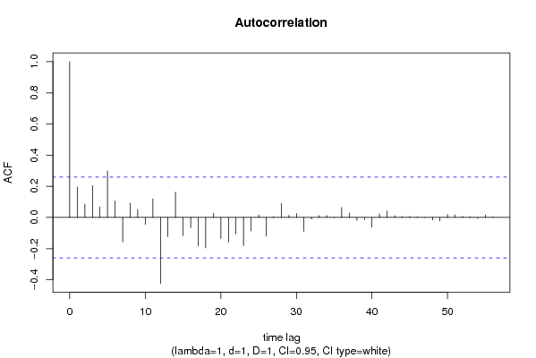
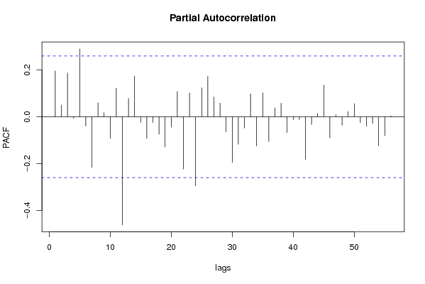
Title produced by software

(Partial) Autocorrelation Function

Date of computation

Sun, 13 Dec 2009 10:47:20 -0700

Cite this page as follows

Statistical Computations at FreeStatistics.org, Office for Research Development and Education, URL https://freestatistics.org/blog/index.php?v=date/2009/Dec/13/t1260726488a7f87p1uap9vgqv.htm/, Retrieved Sun, 28 Apr 2024 06:22:38 +0000

Statistical Computations at FreeStatistics.org, Office for Research Development and Education, URL https://freestatistics.org/blog/index.php?pk=67376, Retrieved Sun, 28 Apr 2024 06:22:38 +0000

QR Codes:

Paste this QR Code to cite your computation.

Original text written by user:

IsPrivate?

No (this computation is public)

User-defined keywords

Estimated Impact

150

Family? (F = Feedback message, R = changed R code, M = changed R Module, P = changed Parameters, D = changed Data)

-     [Univariate Explorative Data Analysis] [Run Sequence gebo...] [2008-12-12 13:32:37] [76963dc1903f0f612b6153510a3818cf]
- R  D  [Univariate Explorative Data Analysis] [Run Sequence gebo...] [2008-12-17 12:14:40] [76963dc1903f0f612b6153510a3818cf]
-         [Univariate Explorative Data Analysis] [Run Sequence Plot...] [2008-12-22 18:19:51] [1ce0d16c8f4225c977b42c8fa93bc163]
- RMP       [(Partial) Autocorrelation Function] [Identifying Integ...] [2009-11-22 12:16:10] [b98453cac15ba1066b407e146608df68]
-   PD        [(Partial) Autocorrelation Function] [W8] [2009-11-25 18:19:32] [315ba876df544ad397193b5931d5f354]
-    D          [(Partial) Autocorrelation Function] [ws8 1.1] [2009-11-27 16:22:27] [95cead3ebb75668735f848316249436a]
-   P             [(Partial) Autocorrelation Function] [ws8.2] [2009-11-27 16:33:59] [95cead3ebb75668735f848316249436a]
-   PD              [(Partial) Autocorrelation Function] [D=1 d=0] [2009-12-13 14:12:45] [95cead3ebb75668735f848316249436a]
-   PD                [(Partial) Autocorrelation Function] [deel2 D=0, d=1] [2009-12-13 17:08:02] [95cead3ebb75668735f848316249436a]
-   P                   [(Partial) Autocorrelation Function] [deel2 D=0 d=2] [2009-12-13 17:09:48] [95cead3ebb75668735f848316249436a]
-   P                       [(Partial) Autocorrelation Function] [deel2 D=1, d=1] [2009-12-13 17:47:20] [95523ebdb89b97dbf680ec91e0b4bca2] [Current]

Feedback Forum

Post a new message

Dataseries X:

Download CSV

Histogram

Boxplots

Summary of computational transaction
Raw Input	view raw input (R code)
Raw Output	view raw output of R engine
Computing time	2 seconds
R Server	'Gwilym Jenkins' @ 72.249.127.135

\begin{tabular}{lllllllll}
\hline
Summary of computational transaction \tabularnewline
Raw Input & view raw input (R code)  \tabularnewline
Raw Output & view raw output of R engine  \tabularnewline
Computing time & 2 seconds \tabularnewline
R Server & 'Gwilym Jenkins' @ 72.249.127.135 \tabularnewline
\hline
\end{tabular}
%Source: https://freestatistics.org/blog/index.php?pk=67376&T=0

[TABLE]
[ROW][C]Summary of computational transaction[/C][/ROW]
[ROW][C]Raw Input[/C][C]view raw input (R code) [/C][/ROW]
[ROW][C]Raw Output[/C][C]view raw output of R engine [/C][/ROW]
[ROW][C]Computing time[/C][C]2 seconds[/C][/ROW]
[ROW][C]R Server[/C][C]'Gwilym Jenkins' @ 72.249.127.135[/C][/ROW]
[/TABLE]
Source: https://freestatistics.org/blog/index.php?pk=67376&T=0

Globally Unique Identifier (entire table): ba.freestatistics.org/blog/index.php?pk=67376&T=0

As an alternative you can also use a QR Code:

The GUIDs for individual cells are displayed in the table below:

Summary of computational transaction
Raw Input	view raw input (R code)
Raw Output	view raw output of R engine
Computing time	2 seconds
R Server	'Gwilym Jenkins' @ 72.249.127.135

Autocorrelation Function
Time lag k	ACF(k)	T-STAT	P-value
1	0.195175	1.4735	0.073053
2	0.086199	0.6508	0.258899
3	0.205287	1.5499	0.063353
4	0.068195	0.5149	0.304319
5	0.298487	2.2535	0.014045
6	0.106227	0.802	0.212943
7	-0.156347	-1.1804	0.121374
8	0.091221	0.6887	0.246902
9	0.051011	0.3851	0.350789
10	-0.044968	-0.3395	0.367741
11	0.119684	0.9036	0.185007
12	-0.423572	-3.1979	0.00113
13	-0.12384	-0.935	0.176873
14	0.162133	1.2241	0.112979
15	-0.118052	-0.8913	0.188265
16	-0.065602	-0.4953	0.311152
17	-0.184306	-1.3915	0.084743
18	-0.196081	-1.4804	0.072139
19	0.026796	0.2023	0.420198
20	-0.135904	-1.026	0.154602
21	-0.158821	-1.1991	0.117731
22	-0.105909	-0.7996	0.213632
23	-0.179979	-1.3588	0.08978
24	-0.086413	-0.6524	0.258383
25	0.016549	0.1249	0.450505
26	-0.119785	-0.9044	0.184806
27	0.005676	0.0429	0.482983
28	0.090026	0.6797	0.249727
29	0.01393	0.1052	0.458305
30	0.026075	0.1969	0.422319
31	-0.08951	-0.6758	0.250954
32	-0.010411	-0.0786	0.468814
33	0.012354	0.0933	0.463009
34	0.012921	0.0976	0.461314
35	-0.003683	-0.0278	0.488958
36	0.064841	0.4895	0.313169
37	0.028865	0.2179	0.414134
38	-0.018471	-0.1395	0.444792
39	-0.014303	-0.108	0.457194
40	-0.061427	-0.4638	0.322293
41	0.022566	0.1704	0.432663
42	0.042361	0.3198	0.375136
43	0.011406	0.0861	0.465838
44	0.006436	0.0486	0.480708
45	0.006475	0.0489	0.48059
46	0.004197	0.0317	0.487415
47	-0.001313	-0.0099	0.496062
48	-0.01539	-0.1162	0.453954
49	-0.023263	-0.1756	0.430603
50	0.01915	0.1446	0.442776
51	0.0173	0.1306	0.448272
52	0.006941	0.0524	0.479195
53	0.005652	0.0427	0.483057
54	-0.005493	-0.0415	0.483532
55	0.01538	0.1161	0.453985
56	0.003324	0.0251	0.490033
57	NA	NA	NA
58	NA	NA	NA
59	NA	NA	NA
60	NA	NA	NA

\begin{tabular}{lllllllll}
\hline
Autocorrelation Function \tabularnewline
Time lag k & ACF(k) & T-STAT & P-value \tabularnewline
1 & 0.195175 & 1.4735 & 0.073053 \tabularnewline
2 & 0.086199 & 0.6508 & 0.258899 \tabularnewline
3 & 0.205287 & 1.5499 & 0.063353 \tabularnewline
4 & 0.068195 & 0.5149 & 0.304319 \tabularnewline
5 & 0.298487 & 2.2535 & 0.014045 \tabularnewline
6 & 0.106227 & 0.802 & 0.212943 \tabularnewline
7 & -0.156347 & -1.1804 & 0.121374 \tabularnewline
8 & 0.091221 & 0.6887 & 0.246902 \tabularnewline
9 & 0.051011 & 0.3851 & 0.350789 \tabularnewline
10 & -0.044968 & -0.3395 & 0.367741 \tabularnewline
11 & 0.119684 & 0.9036 & 0.185007 \tabularnewline
12 & -0.423572 & -3.1979 & 0.00113 \tabularnewline
13 & -0.12384 & -0.935 & 0.176873 \tabularnewline
14 & 0.162133 & 1.2241 & 0.112979 \tabularnewline
15 & -0.118052 & -0.8913 & 0.188265 \tabularnewline
16 & -0.065602 & -0.4953 & 0.311152 \tabularnewline
17 & -0.184306 & -1.3915 & 0.084743 \tabularnewline
18 & -0.196081 & -1.4804 & 0.072139 \tabularnewline
19 & 0.026796 & 0.2023 & 0.420198 \tabularnewline
20 & -0.135904 & -1.026 & 0.154602 \tabularnewline
21 & -0.158821 & -1.1991 & 0.117731 \tabularnewline
22 & -0.105909 & -0.7996 & 0.213632 \tabularnewline
23 & -0.179979 & -1.3588 & 0.08978 \tabularnewline
24 & -0.086413 & -0.6524 & 0.258383 \tabularnewline
25 & 0.016549 & 0.1249 & 0.450505 \tabularnewline
26 & -0.119785 & -0.9044 & 0.184806 \tabularnewline
27 & 0.005676 & 0.0429 & 0.482983 \tabularnewline
28 & 0.090026 & 0.6797 & 0.249727 \tabularnewline
29 & 0.01393 & 0.1052 & 0.458305 \tabularnewline
30 & 0.026075 & 0.1969 & 0.422319 \tabularnewline
31 & -0.08951 & -0.6758 & 0.250954 \tabularnewline
32 & -0.010411 & -0.0786 & 0.468814 \tabularnewline
33 & 0.012354 & 0.0933 & 0.463009 \tabularnewline
34 & 0.012921 & 0.0976 & 0.461314 \tabularnewline
35 & -0.003683 & -0.0278 & 0.488958 \tabularnewline
36 & 0.064841 & 0.4895 & 0.313169 \tabularnewline
37 & 0.028865 & 0.2179 & 0.414134 \tabularnewline
38 & -0.018471 & -0.1395 & 0.444792 \tabularnewline
39 & -0.014303 & -0.108 & 0.457194 \tabularnewline
40 & -0.061427 & -0.4638 & 0.322293 \tabularnewline
41 & 0.022566 & 0.1704 & 0.432663 \tabularnewline
42 & 0.042361 & 0.3198 & 0.375136 \tabularnewline
43 & 0.011406 & 0.0861 & 0.465838 \tabularnewline
44 & 0.006436 & 0.0486 & 0.480708 \tabularnewline
45 & 0.006475 & 0.0489 & 0.48059 \tabularnewline
46 & 0.004197 & 0.0317 & 0.487415 \tabularnewline
47 & -0.001313 & -0.0099 & 0.496062 \tabularnewline
48 & -0.01539 & -0.1162 & 0.453954 \tabularnewline
49 & -0.023263 & -0.1756 & 0.430603 \tabularnewline
50 & 0.01915 & 0.1446 & 0.442776 \tabularnewline
51 & 0.0173 & 0.1306 & 0.448272 \tabularnewline
52 & 0.006941 & 0.0524 & 0.479195 \tabularnewline
53 & 0.005652 & 0.0427 & 0.483057 \tabularnewline
54 & -0.005493 & -0.0415 & 0.483532 \tabularnewline
55 & 0.01538 & 0.1161 & 0.453985 \tabularnewline
56 & 0.003324 & 0.0251 & 0.490033 \tabularnewline
57 & NA & NA & NA \tabularnewline
58 & NA & NA & NA \tabularnewline
59 & NA & NA & NA \tabularnewline
60 & NA & NA & NA \tabularnewline
\hline
\end{tabular}
%Source: https://freestatistics.org/blog/index.php?pk=67376&T=1

[TABLE]
[ROW][C]Autocorrelation Function[/C][/ROW]
[ROW][C]Time lag k[/C][C]ACF(k)[/C][C]T-STAT[/C][C]P-value[/C][/ROW]
[ROW][C]1[/C][C]0.195175[/C][C]1.4735[/C][C]0.073053[/C][/ROW]
[ROW][C]2[/C][C]0.086199[/C][C]0.6508[/C][C]0.258899[/C][/ROW]
[ROW][C]3[/C][C]0.205287[/C][C]1.5499[/C][C]0.063353[/C][/ROW]
[ROW][C]4[/C][C]0.068195[/C][C]0.5149[/C][C]0.304319[/C][/ROW]
[ROW][C]5[/C][C]0.298487[/C][C]2.2535[/C][C]0.014045[/C][/ROW]
[ROW][C]6[/C][C]0.106227[/C][C]0.802[/C][C]0.212943[/C][/ROW]
[ROW][C]7[/C][C]-0.156347[/C][C]-1.1804[/C][C]0.121374[/C][/ROW]
[ROW][C]8[/C][C]0.091221[/C][C]0.6887[/C][C]0.246902[/C][/ROW]
[ROW][C]9[/C][C]0.051011[/C][C]0.3851[/C][C]0.350789[/C][/ROW]
[ROW][C]10[/C][C]-0.044968[/C][C]-0.3395[/C][C]0.367741[/C][/ROW]
[ROW][C]11[/C][C]0.119684[/C][C]0.9036[/C][C]0.185007[/C][/ROW]
[ROW][C]12[/C][C]-0.423572[/C][C]-3.1979[/C][C]0.00113[/C][/ROW]
[ROW][C]13[/C][C]-0.12384[/C][C]-0.935[/C][C]0.176873[/C][/ROW]
[ROW][C]14[/C][C]0.162133[/C][C]1.2241[/C][C]0.112979[/C][/ROW]
[ROW][C]15[/C][C]-0.118052[/C][C]-0.8913[/C][C]0.188265[/C][/ROW]
[ROW][C]16[/C][C]-0.065602[/C][C]-0.4953[/C][C]0.311152[/C][/ROW]
[ROW][C]17[/C][C]-0.184306[/C][C]-1.3915[/C][C]0.084743[/C][/ROW]
[ROW][C]18[/C][C]-0.196081[/C][C]-1.4804[/C][C]0.072139[/C][/ROW]
[ROW][C]19[/C][C]0.026796[/C][C]0.2023[/C][C]0.420198[/C][/ROW]
[ROW][C]20[/C][C]-0.135904[/C][C]-1.026[/C][C]0.154602[/C][/ROW]
[ROW][C]21[/C][C]-0.158821[/C][C]-1.1991[/C][C]0.117731[/C][/ROW]
[ROW][C]22[/C][C]-0.105909[/C][C]-0.7996[/C][C]0.213632[/C][/ROW]
[ROW][C]23[/C][C]-0.179979[/C][C]-1.3588[/C][C]0.08978[/C][/ROW]
[ROW][C]24[/C][C]-0.086413[/C][C]-0.6524[/C][C]0.258383[/C][/ROW]
[ROW][C]25[/C][C]0.016549[/C][C]0.1249[/C][C]0.450505[/C][/ROW]
[ROW][C]26[/C][C]-0.119785[/C][C]-0.9044[/C][C]0.184806[/C][/ROW]
[ROW][C]27[/C][C]0.005676[/C][C]0.0429[/C][C]0.482983[/C][/ROW]
[ROW][C]28[/C][C]0.090026[/C][C]0.6797[/C][C]0.249727[/C][/ROW]
[ROW][C]29[/C][C]0.01393[/C][C]0.1052[/C][C]0.458305[/C][/ROW]
[ROW][C]30[/C][C]0.026075[/C][C]0.1969[/C][C]0.422319[/C][/ROW]
[ROW][C]31[/C][C]-0.08951[/C][C]-0.6758[/C][C]0.250954[/C][/ROW]
[ROW][C]32[/C][C]-0.010411[/C][C]-0.0786[/C][C]0.468814[/C][/ROW]
[ROW][C]33[/C][C]0.012354[/C][C]0.0933[/C][C]0.463009[/C][/ROW]
[ROW][C]34[/C][C]0.012921[/C][C]0.0976[/C][C]0.461314[/C][/ROW]
[ROW][C]35[/C][C]-0.003683[/C][C]-0.0278[/C][C]0.488958[/C][/ROW]
[ROW][C]36[/C][C]0.064841[/C][C]0.4895[/C][C]0.313169[/C][/ROW]
[ROW][C]37[/C][C]0.028865[/C][C]0.2179[/C][C]0.414134[/C][/ROW]
[ROW][C]38[/C][C]-0.018471[/C][C]-0.1395[/C][C]0.444792[/C][/ROW]
[ROW][C]39[/C][C]-0.014303[/C][C]-0.108[/C][C]0.457194[/C][/ROW]
[ROW][C]40[/C][C]-0.061427[/C][C]-0.4638[/C][C]0.322293[/C][/ROW]
[ROW][C]41[/C][C]0.022566[/C][C]0.1704[/C][C]0.432663[/C][/ROW]
[ROW][C]42[/C][C]0.042361[/C][C]0.3198[/C][C]0.375136[/C][/ROW]
[ROW][C]43[/C][C]0.011406[/C][C]0.0861[/C][C]0.465838[/C][/ROW]
[ROW][C]44[/C][C]0.006436[/C][C]0.0486[/C][C]0.480708[/C][/ROW]
[ROW][C]45[/C][C]0.006475[/C][C]0.0489[/C][C]0.48059[/C][/ROW]
[ROW][C]46[/C][C]0.004197[/C][C]0.0317[/C][C]0.487415[/C][/ROW]
[ROW][C]47[/C][C]-0.001313[/C][C]-0.0099[/C][C]0.496062[/C][/ROW]
[ROW][C]48[/C][C]-0.01539[/C][C]-0.1162[/C][C]0.453954[/C][/ROW]
[ROW][C]49[/C][C]-0.023263[/C][C]-0.1756[/C][C]0.430603[/C][/ROW]
[ROW][C]50[/C][C]0.01915[/C][C]0.1446[/C][C]0.442776[/C][/ROW]
[ROW][C]51[/C][C]0.0173[/C][C]0.1306[/C][C]0.448272[/C][/ROW]
[ROW][C]52[/C][C]0.006941[/C][C]0.0524[/C][C]0.479195[/C][/ROW]
[ROW][C]53[/C][C]0.005652[/C][C]0.0427[/C][C]0.483057[/C][/ROW]
[ROW][C]54[/C][C]-0.005493[/C][C]-0.0415[/C][C]0.483532[/C][/ROW]
[ROW][C]55[/C][C]0.01538[/C][C]0.1161[/C][C]0.453985[/C][/ROW]
[ROW][C]56[/C][C]0.003324[/C][C]0.0251[/C][C]0.490033[/C][/ROW]
[ROW][C]57[/C][C]NA[/C][C]NA[/C][C]NA[/C][/ROW]
[ROW][C]58[/C][C]NA[/C][C]NA[/C][C]NA[/C][/ROW]
[ROW][C]59[/C][C]NA[/C][C]NA[/C][C]NA[/C][/ROW]
[ROW][C]60[/C][C]NA[/C][C]NA[/C][C]NA[/C][/ROW]
[/TABLE]
Source: https://freestatistics.org/blog/index.php?pk=67376&T=1

Globally Unique Identifier (entire table): ba.freestatistics.org/blog/index.php?pk=67376&T=1

As an alternative you can also use a QR Code:

The GUIDs for individual cells are displayed in the table below:

Autocorrelation Function
Time lag k	ACF(k)	T-STAT	P-value
1	0.195175	1.4735	0.073053
2	0.086199	0.6508	0.258899
3	0.205287	1.5499	0.063353
4	0.068195	0.5149	0.304319
5	0.298487	2.2535	0.014045
6	0.106227	0.802	0.212943
7	-0.156347	-1.1804	0.121374
8	0.091221	0.6887	0.246902
9	0.051011	0.3851	0.350789
10	-0.044968	-0.3395	0.367741
11	0.119684	0.9036	0.185007
12	-0.423572	-3.1979	0.00113
13	-0.12384	-0.935	0.176873
14	0.162133	1.2241	0.112979
15	-0.118052	-0.8913	0.188265
16	-0.065602	-0.4953	0.311152
17	-0.184306	-1.3915	0.084743
18	-0.196081	-1.4804	0.072139
19	0.026796	0.2023	0.420198
20	-0.135904	-1.026	0.154602
21	-0.158821	-1.1991	0.117731
22	-0.105909	-0.7996	0.213632
23	-0.179979	-1.3588	0.08978
24	-0.086413	-0.6524	0.258383
25	0.016549	0.1249	0.450505
26	-0.119785	-0.9044	0.184806
27	0.005676	0.0429	0.482983
28	0.090026	0.6797	0.249727
29	0.01393	0.1052	0.458305
30	0.026075	0.1969	0.422319
31	-0.08951	-0.6758	0.250954
32	-0.010411	-0.0786	0.468814
33	0.012354	0.0933	0.463009
34	0.012921	0.0976	0.461314
35	-0.003683	-0.0278	0.488958
36	0.064841	0.4895	0.313169
37	0.028865	0.2179	0.414134
38	-0.018471	-0.1395	0.444792
39	-0.014303	-0.108	0.457194
40	-0.061427	-0.4638	0.322293
41	0.022566	0.1704	0.432663
42	0.042361	0.3198	0.375136
43	0.011406	0.0861	0.465838
44	0.006436	0.0486	0.480708
45	0.006475	0.0489	0.48059
46	0.004197	0.0317	0.487415
47	-0.001313	-0.0099	0.496062
48	-0.01539	-0.1162	0.453954
49	-0.023263	-0.1756	0.430603
50	0.01915	0.1446	0.442776
51	0.0173	0.1306	0.448272
52	0.006941	0.0524	0.479195
53	0.005652	0.0427	0.483057
54	-0.005493	-0.0415	0.483532
55	0.01538	0.1161	0.453985
56	0.003324	0.0251	0.490033
57	NA	NA	NA
58	NA	NA	NA
59	NA	NA	NA
60	NA	NA	NA

Partial Autocorrelation Function
Time lag k	PACF(k)	T-STAT	P-value
1	0.195175	1.4735	0.073053
2	0.050011	0.3776	0.353576
3	0.187122	1.4127	0.081585
4	-0.006251	-0.0472	0.48126
5	0.28971	2.1873	0.01642
6	-0.039908	-0.3013	0.382142
7	-0.216009	-1.6308	0.05422
8	0.059709	0.4508	0.326924
9	0.017017	0.1285	0.449112
10	-0.091988	-0.6945	0.245097
11	0.121975	0.9209	0.180494
12	-0.461772	-3.4863	0.000475
13	0.078172	0.5902	0.278698
14	0.17382	1.3123	0.097338
15	-0.024091	-0.1819	0.428159
16	-0.09183	-0.6933	0.245469
17	-0.024966	-0.1885	0.42558
18	-0.074618	-0.5634	0.287701
19	-0.129057	-0.9744	0.166997
20	-0.044105	-0.333	0.370184
21	0.107833	0.8141	0.209482
22	-0.223889	-1.6903	0.048214
23	0.101195	0.764	0.224007
24	-0.295224	-2.2289	0.01489
25	0.123671	0.9337	0.177199
26	0.172512	1.3024	0.099002
27	0.084435	0.6375	0.263185
28	0.058551	0.4421	0.330062
29	-0.064437	-0.4865	0.314243
30	-0.194723	-1.4701	0.073513
31	-0.117853	-0.8898	0.188664
32	-0.04802	-0.3625	0.359142
33	0.097681	0.7375	0.23193
34	-0.12494	-0.9433	0.174761
35	0.1025	0.7739	0.221107
36	-0.105824	-0.799	0.213817
37	0.037948	0.2865	0.387766
38	0.057561	0.4346	0.332755
39	-0.067574	-0.5102	0.305951
40	-0.012371	-0.0934	0.462956
41	-0.011983	-0.0905	0.464116
42	-0.181988	-1.374	0.087413
43	-0.03321	-0.2507	0.401462
44	0.014293	0.1079	0.457223
45	0.134858	1.0182	0.156454
46	-0.090182	-0.6809	0.249358
47	0.008515	0.0643	0.474485
48	-0.036339	-0.2744	0.392402
49	0.02236	0.1688	0.43327
50	0.055687	0.4204	0.337877
51	-0.025021	-0.1889	0.42542
52	-0.04034	-0.3046	0.380904
53	-0.028023	-0.2116	0.4166
54	-0.123563	-0.9329	0.177408
55	-0.080669	-0.609	0.272461
56	0.003871	0.0292	0.488393
57	NA	NA	NA
58	NA	NA	NA
59	NA	NA	NA
60	NA	NA	NA

\begin{tabular}{lllllllll}
\hline
Partial Autocorrelation Function \tabularnewline
Time lag k & PACF(k) & T-STAT & P-value \tabularnewline
1 & 0.195175 & 1.4735 & 0.073053 \tabularnewline
2 & 0.050011 & 0.3776 & 0.353576 \tabularnewline
3 & 0.187122 & 1.4127 & 0.081585 \tabularnewline
4 & -0.006251 & -0.0472 & 0.48126 \tabularnewline
5 & 0.28971 & 2.1873 & 0.01642 \tabularnewline
6 & -0.039908 & -0.3013 & 0.382142 \tabularnewline
7 & -0.216009 & -1.6308 & 0.05422 \tabularnewline
8 & 0.059709 & 0.4508 & 0.326924 \tabularnewline
9 & 0.017017 & 0.1285 & 0.449112 \tabularnewline
10 & -0.091988 & -0.6945 & 0.245097 \tabularnewline
11 & 0.121975 & 0.9209 & 0.180494 \tabularnewline
12 & -0.461772 & -3.4863 & 0.000475 \tabularnewline
13 & 0.078172 & 0.5902 & 0.278698 \tabularnewline
14 & 0.17382 & 1.3123 & 0.097338 \tabularnewline
15 & -0.024091 & -0.1819 & 0.428159 \tabularnewline
16 & -0.09183 & -0.6933 & 0.245469 \tabularnewline
17 & -0.024966 & -0.1885 & 0.42558 \tabularnewline
18 & -0.074618 & -0.5634 & 0.287701 \tabularnewline
19 & -0.129057 & -0.9744 & 0.166997 \tabularnewline
20 & -0.044105 & -0.333 & 0.370184 \tabularnewline
21 & 0.107833 & 0.8141 & 0.209482 \tabularnewline
22 & -0.223889 & -1.6903 & 0.048214 \tabularnewline
23 & 0.101195 & 0.764 & 0.224007 \tabularnewline
24 & -0.295224 & -2.2289 & 0.01489 \tabularnewline
25 & 0.123671 & 0.9337 & 0.177199 \tabularnewline
26 & 0.172512 & 1.3024 & 0.099002 \tabularnewline
27 & 0.084435 & 0.6375 & 0.263185 \tabularnewline
28 & 0.058551 & 0.4421 & 0.330062 \tabularnewline
29 & -0.064437 & -0.4865 & 0.314243 \tabularnewline
30 & -0.194723 & -1.4701 & 0.073513 \tabularnewline
31 & -0.117853 & -0.8898 & 0.188664 \tabularnewline
32 & -0.04802 & -0.3625 & 0.359142 \tabularnewline
33 & 0.097681 & 0.7375 & 0.23193 \tabularnewline
34 & -0.12494 & -0.9433 & 0.174761 \tabularnewline
35 & 0.1025 & 0.7739 & 0.221107 \tabularnewline
36 & -0.105824 & -0.799 & 0.213817 \tabularnewline
37 & 0.037948 & 0.2865 & 0.387766 \tabularnewline
38 & 0.057561 & 0.4346 & 0.332755 \tabularnewline
39 & -0.067574 & -0.5102 & 0.305951 \tabularnewline
40 & -0.012371 & -0.0934 & 0.462956 \tabularnewline
41 & -0.011983 & -0.0905 & 0.464116 \tabularnewline
42 & -0.181988 & -1.374 & 0.087413 \tabularnewline
43 & -0.03321 & -0.2507 & 0.401462 \tabularnewline
44 & 0.014293 & 0.1079 & 0.457223 \tabularnewline
45 & 0.134858 & 1.0182 & 0.156454 \tabularnewline
46 & -0.090182 & -0.6809 & 0.249358 \tabularnewline
47 & 0.008515 & 0.0643 & 0.474485 \tabularnewline
48 & -0.036339 & -0.2744 & 0.392402 \tabularnewline
49 & 0.02236 & 0.1688 & 0.43327 \tabularnewline
50 & 0.055687 & 0.4204 & 0.337877 \tabularnewline
51 & -0.025021 & -0.1889 & 0.42542 \tabularnewline
52 & -0.04034 & -0.3046 & 0.380904 \tabularnewline
53 & -0.028023 & -0.2116 & 0.4166 \tabularnewline
54 & -0.123563 & -0.9329 & 0.177408 \tabularnewline
55 & -0.080669 & -0.609 & 0.272461 \tabularnewline
56 & 0.003871 & 0.0292 & 0.488393 \tabularnewline
57 & NA & NA & NA \tabularnewline
58 & NA & NA & NA \tabularnewline
59 & NA & NA & NA \tabularnewline
60 & NA & NA & NA \tabularnewline
\hline
\end{tabular}
%Source: https://freestatistics.org/blog/index.php?pk=67376&T=2

[TABLE]
[ROW][C]Partial Autocorrelation Function[/C][/ROW]
[ROW][C]Time lag k[/C][C]PACF(k)[/C][C]T-STAT[/C][C]P-value[/C][/ROW]
[ROW][C]1[/C][C]0.195175[/C][C]1.4735[/C][C]0.073053[/C][/ROW]
[ROW][C]2[/C][C]0.050011[/C][C]0.3776[/C][C]0.353576[/C][/ROW]
[ROW][C]3[/C][C]0.187122[/C][C]1.4127[/C][C]0.081585[/C][/ROW]
[ROW][C]4[/C][C]-0.006251[/C][C]-0.0472[/C][C]0.48126[/C][/ROW]
[ROW][C]5[/C][C]0.28971[/C][C]2.1873[/C][C]0.01642[/C][/ROW]
[ROW][C]6[/C][C]-0.039908[/C][C]-0.3013[/C][C]0.382142[/C][/ROW]
[ROW][C]7[/C][C]-0.216009[/C][C]-1.6308[/C][C]0.05422[/C][/ROW]
[ROW][C]8[/C][C]0.059709[/C][C]0.4508[/C][C]0.326924[/C][/ROW]
[ROW][C]9[/C][C]0.017017[/C][C]0.1285[/C][C]0.449112[/C][/ROW]
[ROW][C]10[/C][C]-0.091988[/C][C]-0.6945[/C][C]0.245097[/C][/ROW]
[ROW][C]11[/C][C]0.121975[/C][C]0.9209[/C][C]0.180494[/C][/ROW]
[ROW][C]12[/C][C]-0.461772[/C][C]-3.4863[/C][C]0.000475[/C][/ROW]
[ROW][C]13[/C][C]0.078172[/C][C]0.5902[/C][C]0.278698[/C][/ROW]
[ROW][C]14[/C][C]0.17382[/C][C]1.3123[/C][C]0.097338[/C][/ROW]
[ROW][C]15[/C][C]-0.024091[/C][C]-0.1819[/C][C]0.428159[/C][/ROW]
[ROW][C]16[/C][C]-0.09183[/C][C]-0.6933[/C][C]0.245469[/C][/ROW]
[ROW][C]17[/C][C]-0.024966[/C][C]-0.1885[/C][C]0.42558[/C][/ROW]
[ROW][C]18[/C][C]-0.074618[/C][C]-0.5634[/C][C]0.287701[/C][/ROW]
[ROW][C]19[/C][C]-0.129057[/C][C]-0.9744[/C][C]0.166997[/C][/ROW]
[ROW][C]20[/C][C]-0.044105[/C][C]-0.333[/C][C]0.370184[/C][/ROW]
[ROW][C]21[/C][C]0.107833[/C][C]0.8141[/C][C]0.209482[/C][/ROW]
[ROW][C]22[/C][C]-0.223889[/C][C]-1.6903[/C][C]0.048214[/C][/ROW]
[ROW][C]23[/C][C]0.101195[/C][C]0.764[/C][C]0.224007[/C][/ROW]
[ROW][C]24[/C][C]-0.295224[/C][C]-2.2289[/C][C]0.01489[/C][/ROW]
[ROW][C]25[/C][C]0.123671[/C][C]0.9337[/C][C]0.177199[/C][/ROW]
[ROW][C]26[/C][C]0.172512[/C][C]1.3024[/C][C]0.099002[/C][/ROW]
[ROW][C]27[/C][C]0.084435[/C][C]0.6375[/C][C]0.263185[/C][/ROW]
[ROW][C]28[/C][C]0.058551[/C][C]0.4421[/C][C]0.330062[/C][/ROW]
[ROW][C]29[/C][C]-0.064437[/C][C]-0.4865[/C][C]0.314243[/C][/ROW]
[ROW][C]30[/C][C]-0.194723[/C][C]-1.4701[/C][C]0.073513[/C][/ROW]
[ROW][C]31[/C][C]-0.117853[/C][C]-0.8898[/C][C]0.188664[/C][/ROW]
[ROW][C]32[/C][C]-0.04802[/C][C]-0.3625[/C][C]0.359142[/C][/ROW]
[ROW][C]33[/C][C]0.097681[/C][C]0.7375[/C][C]0.23193[/C][/ROW]
[ROW][C]34[/C][C]-0.12494[/C][C]-0.9433[/C][C]0.174761[/C][/ROW]
[ROW][C]35[/C][C]0.1025[/C][C]0.7739[/C][C]0.221107[/C][/ROW]
[ROW][C]36[/C][C]-0.105824[/C][C]-0.799[/C][C]0.213817[/C][/ROW]
[ROW][C]37[/C][C]0.037948[/C][C]0.2865[/C][C]0.387766[/C][/ROW]
[ROW][C]38[/C][C]0.057561[/C][C]0.4346[/C][C]0.332755[/C][/ROW]
[ROW][C]39[/C][C]-0.067574[/C][C]-0.5102[/C][C]0.305951[/C][/ROW]
[ROW][C]40[/C][C]-0.012371[/C][C]-0.0934[/C][C]0.462956[/C][/ROW]
[ROW][C]41[/C][C]-0.011983[/C][C]-0.0905[/C][C]0.464116[/C][/ROW]
[ROW][C]42[/C][C]-0.181988[/C][C]-1.374[/C][C]0.087413[/C][/ROW]
[ROW][C]43[/C][C]-0.03321[/C][C]-0.2507[/C][C]0.401462[/C][/ROW]
[ROW][C]44[/C][C]0.014293[/C][C]0.1079[/C][C]0.457223[/C][/ROW]
[ROW][C]45[/C][C]0.134858[/C][C]1.0182[/C][C]0.156454[/C][/ROW]
[ROW][C]46[/C][C]-0.090182[/C][C]-0.6809[/C][C]0.249358[/C][/ROW]
[ROW][C]47[/C][C]0.008515[/C][C]0.0643[/C][C]0.474485[/C][/ROW]
[ROW][C]48[/C][C]-0.036339[/C][C]-0.2744[/C][C]0.392402[/C][/ROW]
[ROW][C]49[/C][C]0.02236[/C][C]0.1688[/C][C]0.43327[/C][/ROW]
[ROW][C]50[/C][C]0.055687[/C][C]0.4204[/C][C]0.337877[/C][/ROW]
[ROW][C]51[/C][C]-0.025021[/C][C]-0.1889[/C][C]0.42542[/C][/ROW]
[ROW][C]52[/C][C]-0.04034[/C][C]-0.3046[/C][C]0.380904[/C][/ROW]
[ROW][C]53[/C][C]-0.028023[/C][C]-0.2116[/C][C]0.4166[/C][/ROW]
[ROW][C]54[/C][C]-0.123563[/C][C]-0.9329[/C][C]0.177408[/C][/ROW]
[ROW][C]55[/C][C]-0.080669[/C][C]-0.609[/C][C]0.272461[/C][/ROW]
[ROW][C]56[/C][C]0.003871[/C][C]0.0292[/C][C]0.488393[/C][/ROW]
[ROW][C]57[/C][C]NA[/C][C]NA[/C][C]NA[/C][/ROW]
[ROW][C]58[/C][C]NA[/C][C]NA[/C][C]NA[/C][/ROW]
[ROW][C]59[/C][C]NA[/C][C]NA[/C][C]NA[/C][/ROW]
[ROW][C]60[/C][C]NA[/C][C]NA[/C][C]NA[/C][/ROW]
[/TABLE]
Source: https://freestatistics.org/blog/index.php?pk=67376&T=2

Globally Unique Identifier (entire table): ba.freestatistics.org/blog/index.php?pk=67376&T=2

As an alternative you can also use a QR Code:

The GUIDs for individual cells are displayed in the table below:

Partial Autocorrelation Function
Time lag k	PACF(k)	T-STAT	P-value
1	0.195175	1.4735	0.073053
2	0.050011	0.3776	0.353576
3	0.187122	1.4127	0.081585
4	-0.006251	-0.0472	0.48126
5	0.28971	2.1873	0.01642
6	-0.039908	-0.3013	0.382142
7	-0.216009	-1.6308	0.05422
8	0.059709	0.4508	0.326924
9	0.017017	0.1285	0.449112
10	-0.091988	-0.6945	0.245097
11	0.121975	0.9209	0.180494
12	-0.461772	-3.4863	0.000475
13	0.078172	0.5902	0.278698
14	0.17382	1.3123	0.097338
15	-0.024091	-0.1819	0.428159
16	-0.09183	-0.6933	0.245469
17	-0.024966	-0.1885	0.42558
18	-0.074618	-0.5634	0.287701
19	-0.129057	-0.9744	0.166997
20	-0.044105	-0.333	0.370184
21	0.107833	0.8141	0.209482
22	-0.223889	-1.6903	0.048214
23	0.101195	0.764	0.224007
24	-0.295224	-2.2289	0.01489
25	0.123671	0.9337	0.177199
26	0.172512	1.3024	0.099002
27	0.084435	0.6375	0.263185
28	0.058551	0.4421	0.330062
29	-0.064437	-0.4865	0.314243
30	-0.194723	-1.4701	0.073513
31	-0.117853	-0.8898	0.188664
32	-0.04802	-0.3625	0.359142
33	0.097681	0.7375	0.23193
34	-0.12494	-0.9433	0.174761
35	0.1025	0.7739	0.221107
36	-0.105824	-0.799	0.213817
37	0.037948	0.2865	0.387766
38	0.057561	0.4346	0.332755
39	-0.067574	-0.5102	0.305951
40	-0.012371	-0.0934	0.462956
41	-0.011983	-0.0905	0.464116
42	-0.181988	-1.374	0.087413
43	-0.03321	-0.2507	0.401462
44	0.014293	0.1079	0.457223
45	0.134858	1.0182	0.156454
46	-0.090182	-0.6809	0.249358
47	0.008515	0.0643	0.474485
48	-0.036339	-0.2744	0.392402
49	0.02236	0.1688	0.43327
50	0.055687	0.4204	0.337877
51	-0.025021	-0.1889	0.42542
52	-0.04034	-0.3046	0.380904
53	-0.028023	-0.2116	0.4166
54	-0.123563	-0.9329	0.177408
55	-0.080669	-0.609	0.272461
56	0.003871	0.0292	0.488393
57	NA	NA	NA
58	NA	NA	NA
59	NA	NA	NA
60	NA	NA	NA

Figure 1

PNG link

Postscript link

PDF link

Figure 2

PNG link

Postscript link

PDF link

Parameters (Session):

par1 = 60 ; par2 = 1 ; par3 = 1 ; par4 = 1 ; par5 = 12 ; par6 = White Noise ; par7 = 0.95 ;

Parameters (R input):

par1 = 60 ; par2 = 1 ; par3 = 1 ; par4 = 1 ; par5 = 12 ; par6 = White Noise ; par7 = 0.95 ;

R code (references can be found in the software module):

if (par1 == 'Default') {
par1 = 10*log10(length(x))
} else {
par1 <- as.numeric(par1)
}
par2 <- as.numeric(par2)
par3 <- as.numeric(par3)
par4 <- as.numeric(par4)
par5 <- as.numeric(par5)
if (par6 == 'White Noise') par6 <- 'white' else par6 <- 'ma'
par7 <- as.numeric(par7)
if (par2 == 0) {
x <- log(x)
} else {
x <- (x ^ par2 - 1) / par2
}
if (par3 > 0) x <- diff(x,lag=1,difference=par3)
if (par4 > 0) x <- diff(x,lag=par5,difference=par4)
bitmap(file='pic1.png')
racf <- acf(x, par1, main='Autocorrelation', xlab='time lag', ylab='ACF', ci.type=par6, ci=par7, sub=paste('(lambda=',par2,', d=',par3,', D=',par4,', CI=', par7, ', CI type=',par6,')',sep=''))
dev.off()
bitmap(file='pic2.png')
rpacf <- pacf(x,par1,main='Partial Autocorrelation',xlab='lags',ylab='PACF')
dev.off()
(myacf <- c(racf$acf))
(mypacf <- c(rpacf$acf))
lengthx <- length(x)
sqrtn <- sqrt(lengthx)
load(file='createtable')
a<-table.start()
a<-table.row.start(a)
a<-table.element(a,'Autocorrelation Function',4,TRUE)
a<-table.row.end(a)
a<-table.row.start(a)
a<-table.element(a,'Time lag k',header=TRUE)
a<-table.element(a,hyperlink('basics.htm','ACF(k)','click here for more information about the Autocorrelation Function'),header=TRUE)
a<-table.element(a,'T-STAT',header=TRUE)
a<-table.element(a,'P-value',header=TRUE)
a<-table.row.end(a)
for (i in 2:(par1+1)) {
a<-table.row.start(a)
a<-table.element(a,i-1,header=TRUE)
a<-table.element(a,round(myacf[i],6))
mytstat <- myacf[i]*sqrtn
a<-table.element(a,round(mytstat,4))
a<-table.element(a,round(1-pt(abs(mytstat),lengthx),6))
a<-table.row.end(a)
}
a<-table.end(a)
table.save(a,file='mytable.tab')
a<-table.start()
a<-table.row.start(a)
a<-table.element(a,'Partial Autocorrelation Function',4,TRUE)
a<-table.row.end(a)
a<-table.row.start(a)
a<-table.element(a,'Time lag k',header=TRUE)
a<-table.element(a,hyperlink('basics.htm','PACF(k)','click here for more information about the Partial Autocorrelation Function'),header=TRUE)
a<-table.element(a,'T-STAT',header=TRUE)
a<-table.element(a,'P-value',header=TRUE)
a<-table.row.end(a)
for (i in 1:par1) {
a<-table.row.start(a)
a<-table.element(a,i,header=TRUE)
a<-table.element(a,round(mypacf[i],6))
mytstat <- mypacf[i]*sqrtn
a<-table.element(a,round(mytstat,4))
a<-table.element(a,round(1-pt(abs(mytstat),lengthx),6))
a<-table.row.end(a)
}
a<-table.end(a)
table.save(a,file='mytable1.tab')

Free Statistics

Description of Statistical Computation

Tree of Dependent Computations

Dataset

Tables (Output of Computation)

Figures (Output of Computation)

Input Parameters & R Code