Repository of Reproducible Computations

Free Statistics

of Irreproducible Research!

Author's title

Author

*The author of this computation has been verified*

R Software Module

rwasp_autocorrelation.wasp

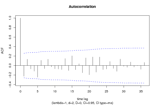
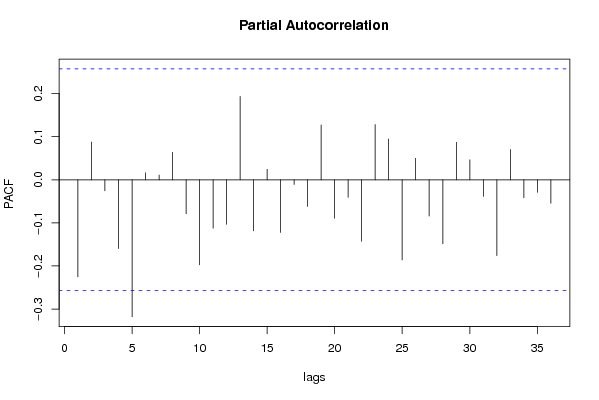
Title produced by software

(Partial) Autocorrelation Function

Date of computation

Sun, 13 Dec 2009 12:11:37 -0700

Cite this page as follows

Statistical Computations at FreeStatistics.org, Office for Research Development and Education, URL https://freestatistics.org/blog/index.php?v=date/2009/Dec/13/t12607315225q38szadm5japwv.htm/, Retrieved Sun, 28 Apr 2024 10:32:40 +0000

Statistical Computations at FreeStatistics.org, Office for Research Development and Education, URL https://freestatistics.org/blog/index.php?pk=67398, Retrieved Sun, 28 Apr 2024 10:32:40 +0000

QR Codes:

Paste this QR Code to cite your computation.

Original text written by user:

IsPrivate?

No (this computation is public)

User-defined keywords

Estimated Impact

121

Family? (F = Feedback message, R = changed R code, M = changed R Module, P = changed Parameters, D = changed Data)

-     [Univariate Explorative Data Analysis] [Run Sequence gebo...] [2008-12-12 13:32:37] [76963dc1903f0f612b6153510a3818cf]
- R  D  [Univariate Explorative Data Analysis] [Run Sequence gebo...] [2008-12-17 12:14:40] [76963dc1903f0f612b6153510a3818cf]
-         [Univariate Explorative Data Analysis] [Run Sequence Plot...] [2008-12-22 18:19:51] [1ce0d16c8f4225c977b42c8fa93bc163]
- RMP       [(Partial) Autocorrelation Function] [Identifying Integ...] [2009-11-22 12:16:10] [b98453cac15ba1066b407e146608df68]
-    D        [(Partial) Autocorrelation Function] [WS8 D=0 en d=0] [2009-11-25 16:06:53] [445b292c553470d9fed8bc2796fd3a00]
-    D          [(Partial) Autocorrelation Function] [ws 8 d=0 D=0] [2009-11-25 20:46:27] [134dc66689e3d457a82860db6471d419]
-    D            [(Partial) Autocorrelation Function] [WS8] [2009-12-13 15:05:34] [85be98bd9ebcfd4d73e77f8552419c9a]
-    D              [(Partial) Autocorrelation Function] [WS9] [2009-12-13 18:59:07] [85be98bd9ebcfd4d73e77f8552419c9a]
-   PD                [(Partial) Autocorrelation Function] [WS9] [2009-12-13 19:01:13] [85be98bd9ebcfd4d73e77f8552419c9a]
-   P                   [(Partial) Autocorrelation Function] [WS9] [2009-12-13 19:03:21] [85be98bd9ebcfd4d73e77f8552419c9a]
-   P                       [(Partial) Autocorrelation Function] [WS9] [2009-12-13 19:11:37] [5cd0e65b1f56b3935a0672588b930e12] [Current]

Feedback Forum

Post a new message

Dataseries X:

Download CSV

Histogram

Boxplots

2.11
2.09
2.05
2.08
2.06
2.06
2.08
2.07
2.06
2.07
2.06
2.09
2.07
2.09
2.28
2.33
2.35
2.52
2.63
2.58
2.70
2.81
2.97
3.04
3.28
3.33
3.50
3.56
3.57
3.69
3.82
3.79
3.96
4.06
4.05
4.03
3.94
4.02
3.88
4.02
4.03
4.09
3.99
4.01
4.01
4.19
4.30
4.27
3.82
3.15
2.49
1.81
1.26
1.06
0.84
0.78
0.70
0.36
0.35
0.36

Summary of computational transaction
Raw Input	view raw input (R code)
Raw Output	view raw output of R engine
Computing time	1 seconds
R Server	'Gwilym Jenkins' @ 72.249.127.135

\begin{tabular}{lllllllll}
\hline
Summary of computational transaction \tabularnewline
Raw Input & view raw input (R code)  \tabularnewline
Raw Output & view raw output of R engine  \tabularnewline
Computing time & 1 seconds \tabularnewline
R Server & 'Gwilym Jenkins' @ 72.249.127.135 \tabularnewline
\hline
\end{tabular}
%Source: https://freestatistics.org/blog/index.php?pk=67398&T=0

[TABLE]
[ROW][C]Summary of computational transaction[/C][/ROW]
[ROW][C]Raw Input[/C][C]view raw input (R code) [/C][/ROW]
[ROW][C]Raw Output[/C][C]view raw output of R engine [/C][/ROW]
[ROW][C]Computing time[/C][C]1 seconds[/C][/ROW]
[ROW][C]R Server[/C][C]'Gwilym Jenkins' @ 72.249.127.135[/C][/ROW]
[/TABLE]
Source: https://freestatistics.org/blog/index.php?pk=67398&T=0

Globally Unique Identifier (entire table): ba.freestatistics.org/blog/index.php?pk=67398&T=0

As an alternative you can also use a QR Code:

The GUIDs for individual cells are displayed in the table below:

Summary of computational transaction
Raw Input	view raw input (R code)
Raw Output	view raw output of R engine
Computing time	1 seconds
R Server	'Gwilym Jenkins' @ 72.249.127.135

Autocorrelation Function
Time lag k	ACF(k)	T-STAT	P-value
1	-0.225056	-1.714	0.045937
2	0.133758	1.0187	0.156294
3	-0.07135	-0.5434	0.294473
4	-0.118962	-0.906	0.184345
5	-0.245429	-1.8691	0.033328
6	0.110923	0.8448	0.200856
7	-0.064845	-0.4938	0.311641
8	0.13398	1.0204	0.155897
9	-0.027178	-0.207	0.418374
10	-0.068471	-0.5215	0.302017
11	-0.073458	-0.5594	0.289007
12	-0.083868	-0.6387	0.262759
13	0.148409	1.1302	0.131512
14	-0.105359	-0.8024	0.2128
15	0.205987	1.5687	0.061073
16	-0.088024	-0.6704	0.25264
17	0.03821	0.291	0.386044
18	-0.151872	-1.1566	0.126085
19	0.162108	1.2346	0.110983
20	-0.194831	-1.4838	0.07164
21	0.181167	1.3797	0.086483
22	-0.139401	-1.0617	0.146398
23	0.181012	1.3785	0.086664
24	-0.086381	-0.6579	0.256615
25	-0.07357	-0.5603	0.288718
26	0.086383	0.6579	0.256611
27	-0.061123	-0.4655	0.32166
28	-0.122371	-0.932	0.177613
29	0.137034	1.0436	0.150495
30	-0.016194	-0.1233	0.451135
31	-0.036633	-0.279	0.390623
32	0.074996	0.5712	0.28505
33	-0.031827	-0.2424	0.404668
34	-0.003649	-0.0278	0.488963
35	-0.079588	-0.6061	0.273399
36	0.06625	0.5045	0.307896

\begin{tabular}{lllllllll}
\hline
Autocorrelation Function \tabularnewline
Time lag k & ACF(k) & T-STAT & P-value \tabularnewline
1 & -0.225056 & -1.714 & 0.045937 \tabularnewline
2 & 0.133758 & 1.0187 & 0.156294 \tabularnewline
3 & -0.07135 & -0.5434 & 0.294473 \tabularnewline
4 & -0.118962 & -0.906 & 0.184345 \tabularnewline
5 & -0.245429 & -1.8691 & 0.033328 \tabularnewline
6 & 0.110923 & 0.8448 & 0.200856 \tabularnewline
7 & -0.064845 & -0.4938 & 0.311641 \tabularnewline
8 & 0.13398 & 1.0204 & 0.155897 \tabularnewline
9 & -0.027178 & -0.207 & 0.418374 \tabularnewline
10 & -0.068471 & -0.5215 & 0.302017 \tabularnewline
11 & -0.073458 & -0.5594 & 0.289007 \tabularnewline
12 & -0.083868 & -0.6387 & 0.262759 \tabularnewline
13 & 0.148409 & 1.1302 & 0.131512 \tabularnewline
14 & -0.105359 & -0.8024 & 0.2128 \tabularnewline
15 & 0.205987 & 1.5687 & 0.061073 \tabularnewline
16 & -0.088024 & -0.6704 & 0.25264 \tabularnewline
17 & 0.03821 & 0.291 & 0.386044 \tabularnewline
18 & -0.151872 & -1.1566 & 0.126085 \tabularnewline
19 & 0.162108 & 1.2346 & 0.110983 \tabularnewline
20 & -0.194831 & -1.4838 & 0.07164 \tabularnewline
21 & 0.181167 & 1.3797 & 0.086483 \tabularnewline
22 & -0.139401 & -1.0617 & 0.146398 \tabularnewline
23 & 0.181012 & 1.3785 & 0.086664 \tabularnewline
24 & -0.086381 & -0.6579 & 0.256615 \tabularnewline
25 & -0.07357 & -0.5603 & 0.288718 \tabularnewline
26 & 0.086383 & 0.6579 & 0.256611 \tabularnewline
27 & -0.061123 & -0.4655 & 0.32166 \tabularnewline
28 & -0.122371 & -0.932 & 0.177613 \tabularnewline
29 & 0.137034 & 1.0436 & 0.150495 \tabularnewline
30 & -0.016194 & -0.1233 & 0.451135 \tabularnewline
31 & -0.036633 & -0.279 & 0.390623 \tabularnewline
32 & 0.074996 & 0.5712 & 0.28505 \tabularnewline
33 & -0.031827 & -0.2424 & 0.404668 \tabularnewline
34 & -0.003649 & -0.0278 & 0.488963 \tabularnewline
35 & -0.079588 & -0.6061 & 0.273399 \tabularnewline
36 & 0.06625 & 0.5045 & 0.307896 \tabularnewline
\hline
\end{tabular}
%Source: https://freestatistics.org/blog/index.php?pk=67398&T=1

[TABLE]
[ROW][C]Autocorrelation Function[/C][/ROW]
[ROW][C]Time lag k[/C][C]ACF(k)[/C][C]T-STAT[/C][C]P-value[/C][/ROW]
[ROW][C]1[/C][C]-0.225056[/C][C]-1.714[/C][C]0.045937[/C][/ROW]
[ROW][C]2[/C][C]0.133758[/C][C]1.0187[/C][C]0.156294[/C][/ROW]
[ROW][C]3[/C][C]-0.07135[/C][C]-0.5434[/C][C]0.294473[/C][/ROW]
[ROW][C]4[/C][C]-0.118962[/C][C]-0.906[/C][C]0.184345[/C][/ROW]
[ROW][C]5[/C][C]-0.245429[/C][C]-1.8691[/C][C]0.033328[/C][/ROW]
[ROW][C]6[/C][C]0.110923[/C][C]0.8448[/C][C]0.200856[/C][/ROW]
[ROW][C]7[/C][C]-0.064845[/C][C]-0.4938[/C][C]0.311641[/C][/ROW]
[ROW][C]8[/C][C]0.13398[/C][C]1.0204[/C][C]0.155897[/C][/ROW]
[ROW][C]9[/C][C]-0.027178[/C][C]-0.207[/C][C]0.418374[/C][/ROW]
[ROW][C]10[/C][C]-0.068471[/C][C]-0.5215[/C][C]0.302017[/C][/ROW]
[ROW][C]11[/C][C]-0.073458[/C][C]-0.5594[/C][C]0.289007[/C][/ROW]
[ROW][C]12[/C][C]-0.083868[/C][C]-0.6387[/C][C]0.262759[/C][/ROW]
[ROW][C]13[/C][C]0.148409[/C][C]1.1302[/C][C]0.131512[/C][/ROW]
[ROW][C]14[/C][C]-0.105359[/C][C]-0.8024[/C][C]0.2128[/C][/ROW]
[ROW][C]15[/C][C]0.205987[/C][C]1.5687[/C][C]0.061073[/C][/ROW]
[ROW][C]16[/C][C]-0.088024[/C][C]-0.6704[/C][C]0.25264[/C][/ROW]
[ROW][C]17[/C][C]0.03821[/C][C]0.291[/C][C]0.386044[/C][/ROW]
[ROW][C]18[/C][C]-0.151872[/C][C]-1.1566[/C][C]0.126085[/C][/ROW]
[ROW][C]19[/C][C]0.162108[/C][C]1.2346[/C][C]0.110983[/C][/ROW]
[ROW][C]20[/C][C]-0.194831[/C][C]-1.4838[/C][C]0.07164[/C][/ROW]
[ROW][C]21[/C][C]0.181167[/C][C]1.3797[/C][C]0.086483[/C][/ROW]
[ROW][C]22[/C][C]-0.139401[/C][C]-1.0617[/C][C]0.146398[/C][/ROW]
[ROW][C]23[/C][C]0.181012[/C][C]1.3785[/C][C]0.086664[/C][/ROW]
[ROW][C]24[/C][C]-0.086381[/C][C]-0.6579[/C][C]0.256615[/C][/ROW]
[ROW][C]25[/C][C]-0.07357[/C][C]-0.5603[/C][C]0.288718[/C][/ROW]
[ROW][C]26[/C][C]0.086383[/C][C]0.6579[/C][C]0.256611[/C][/ROW]
[ROW][C]27[/C][C]-0.061123[/C][C]-0.4655[/C][C]0.32166[/C][/ROW]
[ROW][C]28[/C][C]-0.122371[/C][C]-0.932[/C][C]0.177613[/C][/ROW]
[ROW][C]29[/C][C]0.137034[/C][C]1.0436[/C][C]0.150495[/C][/ROW]
[ROW][C]30[/C][C]-0.016194[/C][C]-0.1233[/C][C]0.451135[/C][/ROW]
[ROW][C]31[/C][C]-0.036633[/C][C]-0.279[/C][C]0.390623[/C][/ROW]
[ROW][C]32[/C][C]0.074996[/C][C]0.5712[/C][C]0.28505[/C][/ROW]
[ROW][C]33[/C][C]-0.031827[/C][C]-0.2424[/C][C]0.404668[/C][/ROW]
[ROW][C]34[/C][C]-0.003649[/C][C]-0.0278[/C][C]0.488963[/C][/ROW]
[ROW][C]35[/C][C]-0.079588[/C][C]-0.6061[/C][C]0.273399[/C][/ROW]
[ROW][C]36[/C][C]0.06625[/C][C]0.5045[/C][C]0.307896[/C][/ROW]
[/TABLE]
Source: https://freestatistics.org/blog/index.php?pk=67398&T=1

Globally Unique Identifier (entire table): ba.freestatistics.org/blog/index.php?pk=67398&T=1

As an alternative you can also use a QR Code:

The GUIDs for individual cells are displayed in the table below:

Autocorrelation Function
Time lag k	ACF(k)	T-STAT	P-value
1	-0.225056	-1.714	0.045937
2	0.133758	1.0187	0.156294
3	-0.07135	-0.5434	0.294473
4	-0.118962	-0.906	0.184345
5	-0.245429	-1.8691	0.033328
6	0.110923	0.8448	0.200856
7	-0.064845	-0.4938	0.311641
8	0.13398	1.0204	0.155897
9	-0.027178	-0.207	0.418374
10	-0.068471	-0.5215	0.302017
11	-0.073458	-0.5594	0.289007
12	-0.083868	-0.6387	0.262759
13	0.148409	1.1302	0.131512
14	-0.105359	-0.8024	0.2128
15	0.205987	1.5687	0.061073
16	-0.088024	-0.6704	0.25264
17	0.03821	0.291	0.386044
18	-0.151872	-1.1566	0.126085
19	0.162108	1.2346	0.110983
20	-0.194831	-1.4838	0.07164
21	0.181167	1.3797	0.086483
22	-0.139401	-1.0617	0.146398
23	0.181012	1.3785	0.086664
24	-0.086381	-0.6579	0.256615
25	-0.07357	-0.5603	0.288718
26	0.086383	0.6579	0.256611
27	-0.061123	-0.4655	0.32166
28	-0.122371	-0.932	0.177613
29	0.137034	1.0436	0.150495
30	-0.016194	-0.1233	0.451135
31	-0.036633	-0.279	0.390623
32	0.074996	0.5712	0.28505
33	-0.031827	-0.2424	0.404668
34	-0.003649	-0.0278	0.488963
35	-0.079588	-0.6061	0.273399
36	0.06625	0.5045	0.307896

Partial Autocorrelation Function
Time lag k	PACF(k)	T-STAT	P-value
1	-0.225056	-1.714	0.045937
2	0.087542	0.6667	0.253803
3	-0.025667	-0.1955	0.422852
4	-0.159577	-1.2153	0.114587
5	-0.317627	-2.419	0.009361
6	0.016324	0.1243	0.450745
7	0.011095	0.0845	0.466477
8	0.06397	0.4872	0.313984
9	-0.078877	-0.6007	0.275187
10	-0.197398	-1.5033	0.069089
11	-0.112243	-0.8548	0.198085
12	-0.103165	-0.7857	0.217626
13	0.193495	1.4736	0.072997
14	-0.118478	-0.9023	0.185314
15	0.024431	0.1861	0.426522
16	-0.122159	-0.9303	0.178028
17	-0.010793	-0.0822	0.467387
18	-0.061833	-0.4709	0.319738
19	0.127309	0.9696	0.168146
20	-0.089171	-0.6791	0.249885
21	-0.040702	-0.31	0.378845
22	-0.142436	-1.0848	0.141258
23	0.128314	0.9772	0.166263
24	0.094509	0.7198	0.237281
25	-0.186131	-1.4175	0.080839
26	0.050021	0.3809	0.352317
27	-0.084203	-0.6413	0.261937
28	-0.148471	-1.1307	0.131414
29	0.08712	0.6635	0.254825
30	0.046432	0.3536	0.362454
31	-0.038164	-0.2906	0.38618
32	-0.175929	-1.3398	0.092762
33	0.070612	0.5378	0.296398
34	-0.041869	-0.3189	0.375488
35	-0.028924	-0.2203	0.413215
36	-0.054115	-0.4121	0.340884

\begin{tabular}{lllllllll}
\hline
Partial Autocorrelation Function \tabularnewline
Time lag k & PACF(k) & T-STAT & P-value \tabularnewline
1 & -0.225056 & -1.714 & 0.045937 \tabularnewline
2 & 0.087542 & 0.6667 & 0.253803 \tabularnewline
3 & -0.025667 & -0.1955 & 0.422852 \tabularnewline
4 & -0.159577 & -1.2153 & 0.114587 \tabularnewline
5 & -0.317627 & -2.419 & 0.009361 \tabularnewline
6 & 0.016324 & 0.1243 & 0.450745 \tabularnewline
7 & 0.011095 & 0.0845 & 0.466477 \tabularnewline
8 & 0.06397 & 0.4872 & 0.313984 \tabularnewline
9 & -0.078877 & -0.6007 & 0.275187 \tabularnewline
10 & -0.197398 & -1.5033 & 0.069089 \tabularnewline
11 & -0.112243 & -0.8548 & 0.198085 \tabularnewline
12 & -0.103165 & -0.7857 & 0.217626 \tabularnewline
13 & 0.193495 & 1.4736 & 0.072997 \tabularnewline
14 & -0.118478 & -0.9023 & 0.185314 \tabularnewline
15 & 0.024431 & 0.1861 & 0.426522 \tabularnewline
16 & -0.122159 & -0.9303 & 0.178028 \tabularnewline
17 & -0.010793 & -0.0822 & 0.467387 \tabularnewline
18 & -0.061833 & -0.4709 & 0.319738 \tabularnewline
19 & 0.127309 & 0.9696 & 0.168146 \tabularnewline
20 & -0.089171 & -0.6791 & 0.249885 \tabularnewline
21 & -0.040702 & -0.31 & 0.378845 \tabularnewline
22 & -0.142436 & -1.0848 & 0.141258 \tabularnewline
23 & 0.128314 & 0.9772 & 0.166263 \tabularnewline
24 & 0.094509 & 0.7198 & 0.237281 \tabularnewline
25 & -0.186131 & -1.4175 & 0.080839 \tabularnewline
26 & 0.050021 & 0.3809 & 0.352317 \tabularnewline
27 & -0.084203 & -0.6413 & 0.261937 \tabularnewline
28 & -0.148471 & -1.1307 & 0.131414 \tabularnewline
29 & 0.08712 & 0.6635 & 0.254825 \tabularnewline
30 & 0.046432 & 0.3536 & 0.362454 \tabularnewline
31 & -0.038164 & -0.2906 & 0.38618 \tabularnewline
32 & -0.175929 & -1.3398 & 0.092762 \tabularnewline
33 & 0.070612 & 0.5378 & 0.296398 \tabularnewline
34 & -0.041869 & -0.3189 & 0.375488 \tabularnewline
35 & -0.028924 & -0.2203 & 0.413215 \tabularnewline
36 & -0.054115 & -0.4121 & 0.340884 \tabularnewline
\hline
\end{tabular}
%Source: https://freestatistics.org/blog/index.php?pk=67398&T=2

[TABLE]
[ROW][C]Partial Autocorrelation Function[/C][/ROW]
[ROW][C]Time lag k[/C][C]PACF(k)[/C][C]T-STAT[/C][C]P-value[/C][/ROW]
[ROW][C]1[/C][C]-0.225056[/C][C]-1.714[/C][C]0.045937[/C][/ROW]
[ROW][C]2[/C][C]0.087542[/C][C]0.6667[/C][C]0.253803[/C][/ROW]
[ROW][C]3[/C][C]-0.025667[/C][C]-0.1955[/C][C]0.422852[/C][/ROW]
[ROW][C]4[/C][C]-0.159577[/C][C]-1.2153[/C][C]0.114587[/C][/ROW]
[ROW][C]5[/C][C]-0.317627[/C][C]-2.419[/C][C]0.009361[/C][/ROW]
[ROW][C]6[/C][C]0.016324[/C][C]0.1243[/C][C]0.450745[/C][/ROW]
[ROW][C]7[/C][C]0.011095[/C][C]0.0845[/C][C]0.466477[/C][/ROW]
[ROW][C]8[/C][C]0.06397[/C][C]0.4872[/C][C]0.313984[/C][/ROW]
[ROW][C]9[/C][C]-0.078877[/C][C]-0.6007[/C][C]0.275187[/C][/ROW]
[ROW][C]10[/C][C]-0.197398[/C][C]-1.5033[/C][C]0.069089[/C][/ROW]
[ROW][C]11[/C][C]-0.112243[/C][C]-0.8548[/C][C]0.198085[/C][/ROW]
[ROW][C]12[/C][C]-0.103165[/C][C]-0.7857[/C][C]0.217626[/C][/ROW]
[ROW][C]13[/C][C]0.193495[/C][C]1.4736[/C][C]0.072997[/C][/ROW]
[ROW][C]14[/C][C]-0.118478[/C][C]-0.9023[/C][C]0.185314[/C][/ROW]
[ROW][C]15[/C][C]0.024431[/C][C]0.1861[/C][C]0.426522[/C][/ROW]
[ROW][C]16[/C][C]-0.122159[/C][C]-0.9303[/C][C]0.178028[/C][/ROW]
[ROW][C]17[/C][C]-0.010793[/C][C]-0.0822[/C][C]0.467387[/C][/ROW]
[ROW][C]18[/C][C]-0.061833[/C][C]-0.4709[/C][C]0.319738[/C][/ROW]
[ROW][C]19[/C][C]0.127309[/C][C]0.9696[/C][C]0.168146[/C][/ROW]
[ROW][C]20[/C][C]-0.089171[/C][C]-0.6791[/C][C]0.249885[/C][/ROW]
[ROW][C]21[/C][C]-0.040702[/C][C]-0.31[/C][C]0.378845[/C][/ROW]
[ROW][C]22[/C][C]-0.142436[/C][C]-1.0848[/C][C]0.141258[/C][/ROW]
[ROW][C]23[/C][C]0.128314[/C][C]0.9772[/C][C]0.166263[/C][/ROW]
[ROW][C]24[/C][C]0.094509[/C][C]0.7198[/C][C]0.237281[/C][/ROW]
[ROW][C]25[/C][C]-0.186131[/C][C]-1.4175[/C][C]0.080839[/C][/ROW]
[ROW][C]26[/C][C]0.050021[/C][C]0.3809[/C][C]0.352317[/C][/ROW]
[ROW][C]27[/C][C]-0.084203[/C][C]-0.6413[/C][C]0.261937[/C][/ROW]
[ROW][C]28[/C][C]-0.148471[/C][C]-1.1307[/C][C]0.131414[/C][/ROW]
[ROW][C]29[/C][C]0.08712[/C][C]0.6635[/C][C]0.254825[/C][/ROW]
[ROW][C]30[/C][C]0.046432[/C][C]0.3536[/C][C]0.362454[/C][/ROW]
[ROW][C]31[/C][C]-0.038164[/C][C]-0.2906[/C][C]0.38618[/C][/ROW]
[ROW][C]32[/C][C]-0.175929[/C][C]-1.3398[/C][C]0.092762[/C][/ROW]
[ROW][C]33[/C][C]0.070612[/C][C]0.5378[/C][C]0.296398[/C][/ROW]
[ROW][C]34[/C][C]-0.041869[/C][C]-0.3189[/C][C]0.375488[/C][/ROW]
[ROW][C]35[/C][C]-0.028924[/C][C]-0.2203[/C][C]0.413215[/C][/ROW]
[ROW][C]36[/C][C]-0.054115[/C][C]-0.4121[/C][C]0.340884[/C][/ROW]
[/TABLE]
Source: https://freestatistics.org/blog/index.php?pk=67398&T=2

Globally Unique Identifier (entire table): ba.freestatistics.org/blog/index.php?pk=67398&T=2

As an alternative you can also use a QR Code:

The GUIDs for individual cells are displayed in the table below:

Partial Autocorrelation Function
Time lag k	PACF(k)	T-STAT	P-value
1	-0.225056	-1.714	0.045937
2	0.087542	0.6667	0.253803
3	-0.025667	-0.1955	0.422852
4	-0.159577	-1.2153	0.114587
5	-0.317627	-2.419	0.009361
6	0.016324	0.1243	0.450745
7	0.011095	0.0845	0.466477
8	0.06397	0.4872	0.313984
9	-0.078877	-0.6007	0.275187
10	-0.197398	-1.5033	0.069089
11	-0.112243	-0.8548	0.198085
12	-0.103165	-0.7857	0.217626
13	0.193495	1.4736	0.072997
14	-0.118478	-0.9023	0.185314
15	0.024431	0.1861	0.426522
16	-0.122159	-0.9303	0.178028
17	-0.010793	-0.0822	0.467387
18	-0.061833	-0.4709	0.319738
19	0.127309	0.9696	0.168146
20	-0.089171	-0.6791	0.249885
21	-0.040702	-0.31	0.378845
22	-0.142436	-1.0848	0.141258
23	0.128314	0.9772	0.166263
24	0.094509	0.7198	0.237281
25	-0.186131	-1.4175	0.080839
26	0.050021	0.3809	0.352317
27	-0.084203	-0.6413	0.261937
28	-0.148471	-1.1307	0.131414
29	0.08712	0.6635	0.254825
30	0.046432	0.3536	0.362454
31	-0.038164	-0.2906	0.38618
32	-0.175929	-1.3398	0.092762
33	0.070612	0.5378	0.296398
34	-0.041869	-0.3189	0.375488
35	-0.028924	-0.2203	0.413215
36	-0.054115	-0.4121	0.340884

Figure 1

PNG link

Postscript link

PDF link

Figure 2

PNG link

Postscript link

PDF link

Parameters (Session):

par1 = 36 ; par2 = 1 ; par3 = 2 ; par4 = 0 ; par5 = 12 ; par6 = MA ; par7 = 0.95 ;

Parameters (R input):

par1 = 36 ; par2 = 1 ; par3 = 2 ; par4 = 0 ; par5 = 12 ; par6 = MA ; par7 = 0.95 ;

R code (references can be found in the software module):

if (par1 == 'Default') {
par1 = 10*log10(length(x))
} else {
par1 <- as.numeric(par1)
}
par2 <- as.numeric(par2)
par3 <- as.numeric(par3)
par4 <- as.numeric(par4)
par5 <- as.numeric(par5)
if (par6 == 'White Noise') par6 <- 'white' else par6 <- 'ma'
par7 <- as.numeric(par7)
if (par2 == 0) {
x <- log(x)
} else {
x <- (x ^ par2 - 1) / par2
}
if (par3 > 0) x <- diff(x,lag=1,difference=par3)
if (par4 > 0) x <- diff(x,lag=par5,difference=par4)
bitmap(file='pic1.png')
racf <- acf(x, par1, main='Autocorrelation', xlab='time lag', ylab='ACF', ci.type=par6, ci=par7, sub=paste('(lambda=',par2,', d=',par3,', D=',par4,', CI=', par7, ', CI type=',par6,')',sep=''))
dev.off()
bitmap(file='pic2.png')
rpacf <- pacf(x,par1,main='Partial Autocorrelation',xlab='lags',ylab='PACF')
dev.off()
(myacf <- c(racf$acf))
(mypacf <- c(rpacf$acf))
lengthx <- length(x)
sqrtn <- sqrt(lengthx)
load(file='createtable')
a<-table.start()
a<-table.row.start(a)
a<-table.element(a,'Autocorrelation Function',4,TRUE)
a<-table.row.end(a)
a<-table.row.start(a)
a<-table.element(a,'Time lag k',header=TRUE)
a<-table.element(a,hyperlink('basics.htm','ACF(k)','click here for more information about the Autocorrelation Function'),header=TRUE)
a<-table.element(a,'T-STAT',header=TRUE)
a<-table.element(a,'P-value',header=TRUE)
a<-table.row.end(a)
for (i in 2:(par1+1)) {
a<-table.row.start(a)
a<-table.element(a,i-1,header=TRUE)
a<-table.element(a,round(myacf[i],6))
mytstat <- myacf[i]*sqrtn
a<-table.element(a,round(mytstat,4))
a<-table.element(a,round(1-pt(abs(mytstat),lengthx),6))
a<-table.row.end(a)
}
a<-table.end(a)
table.save(a,file='mytable.tab')
a<-table.start()
a<-table.row.start(a)
a<-table.element(a,'Partial Autocorrelation Function',4,TRUE)
a<-table.row.end(a)
a<-table.row.start(a)
a<-table.element(a,'Time lag k',header=TRUE)
a<-table.element(a,hyperlink('basics.htm','PACF(k)','click here for more information about the Partial Autocorrelation Function'),header=TRUE)
a<-table.element(a,'T-STAT',header=TRUE)
a<-table.element(a,'P-value',header=TRUE)
a<-table.row.end(a)
for (i in 1:par1) {
a<-table.row.start(a)
a<-table.element(a,i,header=TRUE)
a<-table.element(a,round(mypacf[i],6))
mytstat <- mypacf[i]*sqrtn
a<-table.element(a,round(mytstat,4))
a<-table.element(a,round(1-pt(abs(mytstat),lengthx),6))
a<-table.row.end(a)
}
a<-table.end(a)
table.save(a,file='mytable1.tab')

Free Statistics

Description of Statistical Computation

Tree of Dependent Computations

Dataset

Tables (Output of Computation)

Figures (Output of Computation)

Input Parameters & R Code