Repository of Reproducible Computations

Free Statistics

of Irreproducible Research!

Author's title

Author

*The author of this computation has been verified*

R Software Module

rwasp_autocorrelation.wasp

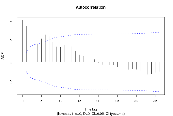
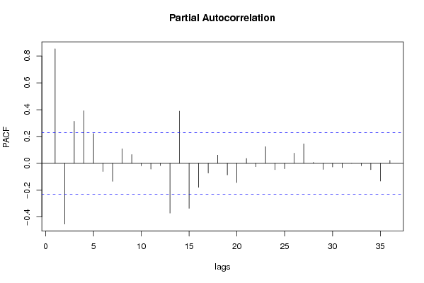
Title produced by software

(Partial) Autocorrelation Function

Date of computation

Thu, 17 Dec 2009 10:07:25 -0700

Cite this page as follows

Statistical Computations at FreeStatistics.org, Office for Research Development and Education, URL https://freestatistics.org/blog/index.php?v=date/2009/Dec/17/t12610697373kxboquj0qo6713.htm/, Retrieved Tue, 30 Apr 2024 06:50:39 +0000

Statistical Computations at FreeStatistics.org, Office for Research Development and Education, URL https://freestatistics.org/blog/index.php?pk=68998, Retrieved Tue, 30 Apr 2024 06:50:39 +0000

QR Codes:

Paste this QR Code to cite your computation.

Original text written by user:

IsPrivate?

No (this computation is public)

User-defined keywords

Estimated Impact

138

Family? (F = Feedback message, R = changed R code, M = changed R Module, P = changed Parameters, D = changed Data)

-     [Univariate Explorative Data Analysis] [Run Sequence gebo...] [2008-12-12 13:32:37] [76963dc1903f0f612b6153510a3818cf]
- R  D  [Univariate Explorative Data Analysis] [Run Sequence gebo...] [2008-12-17 12:14:40] [76963dc1903f0f612b6153510a3818cf]
-         [Univariate Explorative Data Analysis] [Run Sequence Plot...] [2008-12-22 18:19:51] [1ce0d16c8f4225c977b42c8fa93bc163]
- RMP       [(Partial) Autocorrelation Function] [Identifying Integ...] [2009-11-22 12:16:10] [b98453cac15ba1066b407e146608df68]
-    D        [(Partial) Autocorrelation Function] [Partial Correlation ] [2009-11-25 13:28:43] [4395c69e961f9a13a0559fd2f0a72538]
-    D            [(Partial) Autocorrelation Function] [Paper ACF d=D=0 l...] [2009-12-17 17:07:25] [d1081bd6cdf1fed9ed45c42dbd523bf1] [Current]
-   P               [(Partial) Autocorrelation Function] [Paper ACF d= 1 D=...] [2009-12-17 17:12:13] [4395c69e961f9a13a0559fd2f0a72538] 
-   P                 [(Partial) Autocorrelation Function] [Paper ACF d=D=1 l...] [2009-12-17 17:16:30] [4395c69e961f9a13a0559fd2f0a72538] 

Feedback Forum

Post a new message

Dataseries X:

Download CSV

Histogram

Boxplots

7.6
8.3
8.4
8.4
8.4
8.4
8.6
8.9
8.8
8.3
7.5
7.2
7.4
8.8
9.3
9.3
8.7
8.2
8.3
8.5
8.6
8.5
8.2
8.1
7.9
8.6
8.7
8.7
8.5
8.4
8.5
8.7
8.7
8.6
8.5
8.3
8
8.2
8.1
8.1
8
7.9
7.9
8
8
7.9
8
7.7
7.2
7.5
7.3
7
7
7
7.2
7.3
7.1
6.8
6.4
6.1
6.5
7.7
7.9
7.5
6.9
6.6
6.9
7.7
8
8
7.7
7.3
7.4

Summary of computational transaction
Raw Input	view raw input (R code)
Raw Output	view raw output of R engine
Computing time	1 seconds
R Server	'Gwilym Jenkins' @ 72.249.127.135

\begin{tabular}{lllllllll}
\hline
Summary of computational transaction \tabularnewline
Raw Input & view raw input (R code)  \tabularnewline
Raw Output & view raw output of R engine  \tabularnewline
Computing time & 1 seconds \tabularnewline
R Server & 'Gwilym Jenkins' @ 72.249.127.135 \tabularnewline
\hline
\end{tabular}
%Source: https://freestatistics.org/blog/index.php?pk=68998&T=0

[TABLE]
[ROW][C]Summary of computational transaction[/C][/ROW]
[ROW][C]Raw Input[/C][C]view raw input (R code) [/C][/ROW]
[ROW][C]Raw Output[/C][C]view raw output of R engine [/C][/ROW]
[ROW][C]Computing time[/C][C]1 seconds[/C][/ROW]
[ROW][C]R Server[/C][C]'Gwilym Jenkins' @ 72.249.127.135[/C][/ROW]
[/TABLE]
Source: https://freestatistics.org/blog/index.php?pk=68998&T=0

Globally Unique Identifier (entire table): ba.freestatistics.org/blog/index.php?pk=68998&T=0

As an alternative you can also use a QR Code:

The GUIDs for individual cells are displayed in the table below:

Summary of computational transaction
Raw Input	view raw input (R code)
Raw Output	view raw output of R engine
Computing time	1 seconds
R Server	'Gwilym Jenkins' @ 72.249.127.135

Autocorrelation Function
Time lag k	ACF(k)	T-STAT	P-value
1	0.853674	7.2938	0
2	0.606081	5.1784	1e-06
3	0.432859	3.6983	0.000209
4	0.432143	3.6922	0.000213
5	0.555425	4.7456	5e-06
6	0.650199	5.5553	0
7	0.607385	5.1895	1e-06
8	0.475716	4.0645	6e-05
9	0.365624	3.1239	0.00128
10	0.349605	2.987	0.001917
11	0.405859	3.4677	0.000442
12	0.449741	3.8426	0.000129
13	0.365739	3.1249	0.001276
14	0.259052	2.2133	0.015
15	0.172388	1.4729	0.072541
16	0.135164	1.1548	0.125961
17	0.131716	1.1254	0.132057
18	0.115759	0.989	0.162953
19	0.058946	0.5036	0.308016
20	-0.010438	-0.0892	0.464591
21	-0.058891	-0.5032	0.308182
22	-0.076562	-0.6541	0.257538
23	-0.068804	-0.5879	0.279219
24	-0.064115	-0.5478	0.29275
25	-0.118654	-1.0138	0.157018
26	-0.157158	-1.3428	0.091755
27	-0.177937	-1.5203	0.066379
28	-0.17679	-1.5105	0.067617
29	-0.166574	-1.4232	0.079467
30	-0.175005	-1.4952	0.069581
31	-0.21772	-1.8602	0.033443
32	-0.268286	-2.2922	0.012388
33	-0.292779	-2.5015	0.007304
34	-0.281843	-2.4081	0.009282
35	-0.24784	-2.1175	0.01881
36	-0.225625	-1.9277	0.028889

\begin{tabular}{lllllllll}
\hline
Autocorrelation Function \tabularnewline
Time lag k & ACF(k) & T-STAT & P-value \tabularnewline
1 & 0.853674 & 7.2938 & 0 \tabularnewline
2 & 0.606081 & 5.1784 & 1e-06 \tabularnewline
3 & 0.432859 & 3.6983 & 0.000209 \tabularnewline
4 & 0.432143 & 3.6922 & 0.000213 \tabularnewline
5 & 0.555425 & 4.7456 & 5e-06 \tabularnewline
6 & 0.650199 & 5.5553 & 0 \tabularnewline
7 & 0.607385 & 5.1895 & 1e-06 \tabularnewline
8 & 0.475716 & 4.0645 & 6e-05 \tabularnewline
9 & 0.365624 & 3.1239 & 0.00128 \tabularnewline
10 & 0.349605 & 2.987 & 0.001917 \tabularnewline
11 & 0.405859 & 3.4677 & 0.000442 \tabularnewline
12 & 0.449741 & 3.8426 & 0.000129 \tabularnewline
13 & 0.365739 & 3.1249 & 0.001276 \tabularnewline
14 & 0.259052 & 2.2133 & 0.015 \tabularnewline
15 & 0.172388 & 1.4729 & 0.072541 \tabularnewline
16 & 0.135164 & 1.1548 & 0.125961 \tabularnewline
17 & 0.131716 & 1.1254 & 0.132057 \tabularnewline
18 & 0.115759 & 0.989 & 0.162953 \tabularnewline
19 & 0.058946 & 0.5036 & 0.308016 \tabularnewline
20 & -0.010438 & -0.0892 & 0.464591 \tabularnewline
21 & -0.058891 & -0.5032 & 0.308182 \tabularnewline
22 & -0.076562 & -0.6541 & 0.257538 \tabularnewline
23 & -0.068804 & -0.5879 & 0.279219 \tabularnewline
24 & -0.064115 & -0.5478 & 0.29275 \tabularnewline
25 & -0.118654 & -1.0138 & 0.157018 \tabularnewline
26 & -0.157158 & -1.3428 & 0.091755 \tabularnewline
27 & -0.177937 & -1.5203 & 0.066379 \tabularnewline
28 & -0.17679 & -1.5105 & 0.067617 \tabularnewline
29 & -0.166574 & -1.4232 & 0.079467 \tabularnewline
30 & -0.175005 & -1.4952 & 0.069581 \tabularnewline
31 & -0.21772 & -1.8602 & 0.033443 \tabularnewline
32 & -0.268286 & -2.2922 & 0.012388 \tabularnewline
33 & -0.292779 & -2.5015 & 0.007304 \tabularnewline
34 & -0.281843 & -2.4081 & 0.009282 \tabularnewline
35 & -0.24784 & -2.1175 & 0.01881 \tabularnewline
36 & -0.225625 & -1.9277 & 0.028889 \tabularnewline
\hline
\end{tabular}
%Source: https://freestatistics.org/blog/index.php?pk=68998&T=1

[TABLE]
[ROW][C]Autocorrelation Function[/C][/ROW]
[ROW][C]Time lag k[/C][C]ACF(k)[/C][C]T-STAT[/C][C]P-value[/C][/ROW]
[ROW][C]1[/C][C]0.853674[/C][C]7.2938[/C][C]0[/C][/ROW]
[ROW][C]2[/C][C]0.606081[/C][C]5.1784[/C][C]1e-06[/C][/ROW]
[ROW][C]3[/C][C]0.432859[/C][C]3.6983[/C][C]0.000209[/C][/ROW]
[ROW][C]4[/C][C]0.432143[/C][C]3.6922[/C][C]0.000213[/C][/ROW]
[ROW][C]5[/C][C]0.555425[/C][C]4.7456[/C][C]5e-06[/C][/ROW]
[ROW][C]6[/C][C]0.650199[/C][C]5.5553[/C][C]0[/C][/ROW]
[ROW][C]7[/C][C]0.607385[/C][C]5.1895[/C][C]1e-06[/C][/ROW]
[ROW][C]8[/C][C]0.475716[/C][C]4.0645[/C][C]6e-05[/C][/ROW]
[ROW][C]9[/C][C]0.365624[/C][C]3.1239[/C][C]0.00128[/C][/ROW]
[ROW][C]10[/C][C]0.349605[/C][C]2.987[/C][C]0.001917[/C][/ROW]
[ROW][C]11[/C][C]0.405859[/C][C]3.4677[/C][C]0.000442[/C][/ROW]
[ROW][C]12[/C][C]0.449741[/C][C]3.8426[/C][C]0.000129[/C][/ROW]
[ROW][C]13[/C][C]0.365739[/C][C]3.1249[/C][C]0.001276[/C][/ROW]
[ROW][C]14[/C][C]0.259052[/C][C]2.2133[/C][C]0.015[/C][/ROW]
[ROW][C]15[/C][C]0.172388[/C][C]1.4729[/C][C]0.072541[/C][/ROW]
[ROW][C]16[/C][C]0.135164[/C][C]1.1548[/C][C]0.125961[/C][/ROW]
[ROW][C]17[/C][C]0.131716[/C][C]1.1254[/C][C]0.132057[/C][/ROW]
[ROW][C]18[/C][C]0.115759[/C][C]0.989[/C][C]0.162953[/C][/ROW]
[ROW][C]19[/C][C]0.058946[/C][C]0.5036[/C][C]0.308016[/C][/ROW]
[ROW][C]20[/C][C]-0.010438[/C][C]-0.0892[/C][C]0.464591[/C][/ROW]
[ROW][C]21[/C][C]-0.058891[/C][C]-0.5032[/C][C]0.308182[/C][/ROW]
[ROW][C]22[/C][C]-0.076562[/C][C]-0.6541[/C][C]0.257538[/C][/ROW]
[ROW][C]23[/C][C]-0.068804[/C][C]-0.5879[/C][C]0.279219[/C][/ROW]
[ROW][C]24[/C][C]-0.064115[/C][C]-0.5478[/C][C]0.29275[/C][/ROW]
[ROW][C]25[/C][C]-0.118654[/C][C]-1.0138[/C][C]0.157018[/C][/ROW]
[ROW][C]26[/C][C]-0.157158[/C][C]-1.3428[/C][C]0.091755[/C][/ROW]
[ROW][C]27[/C][C]-0.177937[/C][C]-1.5203[/C][C]0.066379[/C][/ROW]
[ROW][C]28[/C][C]-0.17679[/C][C]-1.5105[/C][C]0.067617[/C][/ROW]
[ROW][C]29[/C][C]-0.166574[/C][C]-1.4232[/C][C]0.079467[/C][/ROW]
[ROW][C]30[/C][C]-0.175005[/C][C]-1.4952[/C][C]0.069581[/C][/ROW]
[ROW][C]31[/C][C]-0.21772[/C][C]-1.8602[/C][C]0.033443[/C][/ROW]
[ROW][C]32[/C][C]-0.268286[/C][C]-2.2922[/C][C]0.012388[/C][/ROW]
[ROW][C]33[/C][C]-0.292779[/C][C]-2.5015[/C][C]0.007304[/C][/ROW]
[ROW][C]34[/C][C]-0.281843[/C][C]-2.4081[/C][C]0.009282[/C][/ROW]
[ROW][C]35[/C][C]-0.24784[/C][C]-2.1175[/C][C]0.01881[/C][/ROW]
[ROW][C]36[/C][C]-0.225625[/C][C]-1.9277[/C][C]0.028889[/C][/ROW]
[/TABLE]
Source: https://freestatistics.org/blog/index.php?pk=68998&T=1

Globally Unique Identifier (entire table): ba.freestatistics.org/blog/index.php?pk=68998&T=1

As an alternative you can also use a QR Code:

The GUIDs for individual cells are displayed in the table below:

Autocorrelation Function
Time lag k	ACF(k)	T-STAT	P-value
1	0.853674	7.2938	0
2	0.606081	5.1784	1e-06
3	0.432859	3.6983	0.000209
4	0.432143	3.6922	0.000213
5	0.555425	4.7456	5e-06
6	0.650199	5.5553	0
7	0.607385	5.1895	1e-06
8	0.475716	4.0645	6e-05
9	0.365624	3.1239	0.00128
10	0.349605	2.987	0.001917
11	0.405859	3.4677	0.000442
12	0.449741	3.8426	0.000129
13	0.365739	3.1249	0.001276
14	0.259052	2.2133	0.015
15	0.172388	1.4729	0.072541
16	0.135164	1.1548	0.125961
17	0.131716	1.1254	0.132057
18	0.115759	0.989	0.162953
19	0.058946	0.5036	0.308016
20	-0.010438	-0.0892	0.464591
21	-0.058891	-0.5032	0.308182
22	-0.076562	-0.6541	0.257538
23	-0.068804	-0.5879	0.279219
24	-0.064115	-0.5478	0.29275
25	-0.118654	-1.0138	0.157018
26	-0.157158	-1.3428	0.091755
27	-0.177937	-1.5203	0.066379
28	-0.17679	-1.5105	0.067617
29	-0.166574	-1.4232	0.079467
30	-0.175005	-1.4952	0.069581
31	-0.21772	-1.8602	0.033443
32	-0.268286	-2.2922	0.012388
33	-0.292779	-2.5015	0.007304
34	-0.281843	-2.4081	0.009282
35	-0.24784	-2.1175	0.01881
36	-0.225625	-1.9277	0.028889

Partial Autocorrelation Function
Time lag k	PACF(k)	T-STAT	P-value
1	0.853674	7.2938	0
2	-0.452283	-3.8643	0.00012
3	0.313116	2.6753	0.004606
4	0.392044	3.3496	0.000642
5	0.221472	1.8923	0.031211
6	-0.060863	-0.52	0.302314
7	-0.134399	-1.1483	0.127296
8	0.108063	0.9233	0.179449
9	0.065737	0.5617	0.288036
10	-0.018226	-0.1557	0.438339
11	-0.043409	-0.3709	0.355897
12	-0.016852	-0.144	0.442956
13	-0.370513	-3.1657	0.001129
14	0.388867	3.3225	0.000698
15	-0.334888	-2.8613	0.00275
16	-0.179096	-1.5302	0.065145
17	-0.072149	-0.6164	0.269761
18	0.060863	0.52	0.302312
19	-0.086213	-0.7366	0.231861
20	-0.143355	-1.2248	0.11229
21	0.036507	0.3119	0.377996
22	-0.025199	-0.2153	0.415066
23	0.124245	1.0615	0.14597
24	-0.047277	-0.4039	0.343722
25	-0.040682	-0.3476	0.364575
26	0.076015	0.6495	0.259035
27	0.145103	1.2398	0.109517
28	0.006877	0.0588	0.476653
29	-0.045482	-0.3886	0.349351
30	-0.027669	-0.2364	0.406891
31	-0.031792	-0.2716	0.393337
32	0.000592	0.0051	0.497989
33	-0.017263	-0.1475	0.441575
34	-0.047336	-0.4044	0.343536
35	-0.132084	-1.1285	0.131396
36	0.022256	0.1902	0.424858

\begin{tabular}{lllllllll}
\hline
Partial Autocorrelation Function \tabularnewline
Time lag k & PACF(k) & T-STAT & P-value \tabularnewline
1 & 0.853674 & 7.2938 & 0 \tabularnewline
2 & -0.452283 & -3.8643 & 0.00012 \tabularnewline
3 & 0.313116 & 2.6753 & 0.004606 \tabularnewline
4 & 0.392044 & 3.3496 & 0.000642 \tabularnewline
5 & 0.221472 & 1.8923 & 0.031211 \tabularnewline
6 & -0.060863 & -0.52 & 0.302314 \tabularnewline
7 & -0.134399 & -1.1483 & 0.127296 \tabularnewline
8 & 0.108063 & 0.9233 & 0.179449 \tabularnewline
9 & 0.065737 & 0.5617 & 0.288036 \tabularnewline
10 & -0.018226 & -0.1557 & 0.438339 \tabularnewline
11 & -0.043409 & -0.3709 & 0.355897 \tabularnewline
12 & -0.016852 & -0.144 & 0.442956 \tabularnewline
13 & -0.370513 & -3.1657 & 0.001129 \tabularnewline
14 & 0.388867 & 3.3225 & 0.000698 \tabularnewline
15 & -0.334888 & -2.8613 & 0.00275 \tabularnewline
16 & -0.179096 & -1.5302 & 0.065145 \tabularnewline
17 & -0.072149 & -0.6164 & 0.269761 \tabularnewline
18 & 0.060863 & 0.52 & 0.302312 \tabularnewline
19 & -0.086213 & -0.7366 & 0.231861 \tabularnewline
20 & -0.143355 & -1.2248 & 0.11229 \tabularnewline
21 & 0.036507 & 0.3119 & 0.377996 \tabularnewline
22 & -0.025199 & -0.2153 & 0.415066 \tabularnewline
23 & 0.124245 & 1.0615 & 0.14597 \tabularnewline
24 & -0.047277 & -0.4039 & 0.343722 \tabularnewline
25 & -0.040682 & -0.3476 & 0.364575 \tabularnewline
26 & 0.076015 & 0.6495 & 0.259035 \tabularnewline
27 & 0.145103 & 1.2398 & 0.109517 \tabularnewline
28 & 0.006877 & 0.0588 & 0.476653 \tabularnewline
29 & -0.045482 & -0.3886 & 0.349351 \tabularnewline
30 & -0.027669 & -0.2364 & 0.406891 \tabularnewline
31 & -0.031792 & -0.2716 & 0.393337 \tabularnewline
32 & 0.000592 & 0.0051 & 0.497989 \tabularnewline
33 & -0.017263 & -0.1475 & 0.441575 \tabularnewline
34 & -0.047336 & -0.4044 & 0.343536 \tabularnewline
35 & -0.132084 & -1.1285 & 0.131396 \tabularnewline
36 & 0.022256 & 0.1902 & 0.424858 \tabularnewline
\hline
\end{tabular}
%Source: https://freestatistics.org/blog/index.php?pk=68998&T=2

[TABLE]
[ROW][C]Partial Autocorrelation Function[/C][/ROW]
[ROW][C]Time lag k[/C][C]PACF(k)[/C][C]T-STAT[/C][C]P-value[/C][/ROW]
[ROW][C]1[/C][C]0.853674[/C][C]7.2938[/C][C]0[/C][/ROW]
[ROW][C]2[/C][C]-0.452283[/C][C]-3.8643[/C][C]0.00012[/C][/ROW]
[ROW][C]3[/C][C]0.313116[/C][C]2.6753[/C][C]0.004606[/C][/ROW]
[ROW][C]4[/C][C]0.392044[/C][C]3.3496[/C][C]0.000642[/C][/ROW]
[ROW][C]5[/C][C]0.221472[/C][C]1.8923[/C][C]0.031211[/C][/ROW]
[ROW][C]6[/C][C]-0.060863[/C][C]-0.52[/C][C]0.302314[/C][/ROW]
[ROW][C]7[/C][C]-0.134399[/C][C]-1.1483[/C][C]0.127296[/C][/ROW]
[ROW][C]8[/C][C]0.108063[/C][C]0.9233[/C][C]0.179449[/C][/ROW]
[ROW][C]9[/C][C]0.065737[/C][C]0.5617[/C][C]0.288036[/C][/ROW]
[ROW][C]10[/C][C]-0.018226[/C][C]-0.1557[/C][C]0.438339[/C][/ROW]
[ROW][C]11[/C][C]-0.043409[/C][C]-0.3709[/C][C]0.355897[/C][/ROW]
[ROW][C]12[/C][C]-0.016852[/C][C]-0.144[/C][C]0.442956[/C][/ROW]
[ROW][C]13[/C][C]-0.370513[/C][C]-3.1657[/C][C]0.001129[/C][/ROW]
[ROW][C]14[/C][C]0.388867[/C][C]3.3225[/C][C]0.000698[/C][/ROW]
[ROW][C]15[/C][C]-0.334888[/C][C]-2.8613[/C][C]0.00275[/C][/ROW]
[ROW][C]16[/C][C]-0.179096[/C][C]-1.5302[/C][C]0.065145[/C][/ROW]
[ROW][C]17[/C][C]-0.072149[/C][C]-0.6164[/C][C]0.269761[/C][/ROW]
[ROW][C]18[/C][C]0.060863[/C][C]0.52[/C][C]0.302312[/C][/ROW]
[ROW][C]19[/C][C]-0.086213[/C][C]-0.7366[/C][C]0.231861[/C][/ROW]
[ROW][C]20[/C][C]-0.143355[/C][C]-1.2248[/C][C]0.11229[/C][/ROW]
[ROW][C]21[/C][C]0.036507[/C][C]0.3119[/C][C]0.377996[/C][/ROW]
[ROW][C]22[/C][C]-0.025199[/C][C]-0.2153[/C][C]0.415066[/C][/ROW]
[ROW][C]23[/C][C]0.124245[/C][C]1.0615[/C][C]0.14597[/C][/ROW]
[ROW][C]24[/C][C]-0.047277[/C][C]-0.4039[/C][C]0.343722[/C][/ROW]
[ROW][C]25[/C][C]-0.040682[/C][C]-0.3476[/C][C]0.364575[/C][/ROW]
[ROW][C]26[/C][C]0.076015[/C][C]0.6495[/C][C]0.259035[/C][/ROW]
[ROW][C]27[/C][C]0.145103[/C][C]1.2398[/C][C]0.109517[/C][/ROW]
[ROW][C]28[/C][C]0.006877[/C][C]0.0588[/C][C]0.476653[/C][/ROW]
[ROW][C]29[/C][C]-0.045482[/C][C]-0.3886[/C][C]0.349351[/C][/ROW]
[ROW][C]30[/C][C]-0.027669[/C][C]-0.2364[/C][C]0.406891[/C][/ROW]
[ROW][C]31[/C][C]-0.031792[/C][C]-0.2716[/C][C]0.393337[/C][/ROW]
[ROW][C]32[/C][C]0.000592[/C][C]0.0051[/C][C]0.497989[/C][/ROW]
[ROW][C]33[/C][C]-0.017263[/C][C]-0.1475[/C][C]0.441575[/C][/ROW]
[ROW][C]34[/C][C]-0.047336[/C][C]-0.4044[/C][C]0.343536[/C][/ROW]
[ROW][C]35[/C][C]-0.132084[/C][C]-1.1285[/C][C]0.131396[/C][/ROW]
[ROW][C]36[/C][C]0.022256[/C][C]0.1902[/C][C]0.424858[/C][/ROW]
[/TABLE]
Source: https://freestatistics.org/blog/index.php?pk=68998&T=2

Globally Unique Identifier (entire table): ba.freestatistics.org/blog/index.php?pk=68998&T=2

As an alternative you can also use a QR Code:

The GUIDs for individual cells are displayed in the table below:

Partial Autocorrelation Function
Time lag k	PACF(k)	T-STAT	P-value
1	0.853674	7.2938	0
2	-0.452283	-3.8643	0.00012
3	0.313116	2.6753	0.004606
4	0.392044	3.3496	0.000642
5	0.221472	1.8923	0.031211
6	-0.060863	-0.52	0.302314
7	-0.134399	-1.1483	0.127296
8	0.108063	0.9233	0.179449
9	0.065737	0.5617	0.288036
10	-0.018226	-0.1557	0.438339
11	-0.043409	-0.3709	0.355897
12	-0.016852	-0.144	0.442956
13	-0.370513	-3.1657	0.001129
14	0.388867	3.3225	0.000698
15	-0.334888	-2.8613	0.00275
16	-0.179096	-1.5302	0.065145
17	-0.072149	-0.6164	0.269761
18	0.060863	0.52	0.302312
19	-0.086213	-0.7366	0.231861
20	-0.143355	-1.2248	0.11229
21	0.036507	0.3119	0.377996
22	-0.025199	-0.2153	0.415066
23	0.124245	1.0615	0.14597
24	-0.047277	-0.4039	0.343722
25	-0.040682	-0.3476	0.364575
26	0.076015	0.6495	0.259035
27	0.145103	1.2398	0.109517
28	0.006877	0.0588	0.476653
29	-0.045482	-0.3886	0.349351
30	-0.027669	-0.2364	0.406891
31	-0.031792	-0.2716	0.393337
32	0.000592	0.0051	0.497989
33	-0.017263	-0.1475	0.441575
34	-0.047336	-0.4044	0.343536
35	-0.132084	-1.1285	0.131396
36	0.022256	0.1902	0.424858

Figure 1

PNG link

Postscript link

PDF link

Figure 2

PNG link

Postscript link

PDF link

Parameters (Session):

par1 = 36 ; par2 = 1 ; par3 = 0 ; par4 = 0 ; par5 = 12 ; par6 = MA ; par7 = 0.95 ;

Parameters (R input):

par1 = 36 ; par2 = 1 ; par3 = 0 ; par4 = 0 ; par5 = 12 ; par6 = MA ; par7 = 0.95 ;

R code (references can be found in the software module):

if (par1 == 'Default') {
par1 = 10*log10(length(x))
} else {
par1 <- as.numeric(par1)
}
par2 <- as.numeric(par2)
par3 <- as.numeric(par3)
par4 <- as.numeric(par4)
par5 <- as.numeric(par5)
if (par6 == 'White Noise') par6 <- 'white' else par6 <- 'ma'
par7 <- as.numeric(par7)
if (par2 == 0) {
x <- log(x)
} else {
x <- (x ^ par2 - 1) / par2
}
if (par3 > 0) x <- diff(x,lag=1,difference=par3)
if (par4 > 0) x <- diff(x,lag=par5,difference=par4)
bitmap(file='pic1.png')
racf <- acf(x, par1, main='Autocorrelation', xlab='time lag', ylab='ACF', ci.type=par6, ci=par7, sub=paste('(lambda=',par2,', d=',par3,', D=',par4,', CI=', par7, ', CI type=',par6,')',sep=''))
dev.off()
bitmap(file='pic2.png')
rpacf <- pacf(x,par1,main='Partial Autocorrelation',xlab='lags',ylab='PACF')
dev.off()
(myacf <- c(racf$acf))
(mypacf <- c(rpacf$acf))
lengthx <- length(x)
sqrtn <- sqrt(lengthx)
load(file='createtable')
a<-table.start()
a<-table.row.start(a)
a<-table.element(a,'Autocorrelation Function',4,TRUE)
a<-table.row.end(a)
a<-table.row.start(a)
a<-table.element(a,'Time lag k',header=TRUE)
a<-table.element(a,hyperlink('basics.htm','ACF(k)','click here for more information about the Autocorrelation Function'),header=TRUE)
a<-table.element(a,'T-STAT',header=TRUE)
a<-table.element(a,'P-value',header=TRUE)
a<-table.row.end(a)
for (i in 2:(par1+1)) {
a<-table.row.start(a)
a<-table.element(a,i-1,header=TRUE)
a<-table.element(a,round(myacf[i],6))
mytstat <- myacf[i]*sqrtn
a<-table.element(a,round(mytstat,4))
a<-table.element(a,round(1-pt(abs(mytstat),lengthx),6))
a<-table.row.end(a)
}
a<-table.end(a)
table.save(a,file='mytable.tab')
a<-table.start()
a<-table.row.start(a)
a<-table.element(a,'Partial Autocorrelation Function',4,TRUE)
a<-table.row.end(a)
a<-table.row.start(a)
a<-table.element(a,'Time lag k',header=TRUE)
a<-table.element(a,hyperlink('basics.htm','PACF(k)','click here for more information about the Partial Autocorrelation Function'),header=TRUE)
a<-table.element(a,'T-STAT',header=TRUE)
a<-table.element(a,'P-value',header=TRUE)
a<-table.row.end(a)
for (i in 1:par1) {
a<-table.row.start(a)
a<-table.element(a,i,header=TRUE)
a<-table.element(a,round(mypacf[i],6))
mytstat <- mypacf[i]*sqrtn
a<-table.element(a,round(mytstat,4))
a<-table.element(a,round(1-pt(abs(mytstat),lengthx),6))
a<-table.row.end(a)
}
a<-table.end(a)
table.save(a,file='mytable1.tab')

Free Statistics

Description of Statistical Computation

Tree of Dependent Computations

Dataset

Tables (Output of Computation)

Figures (Output of Computation)

Input Parameters & R Code