Repository of Reproducible Computations

Free Statistics

of Irreproducible Research!

Author's title

Author

*The author of this computation has been verified*

R Software Module

rwasp_autocorrelation.wasp

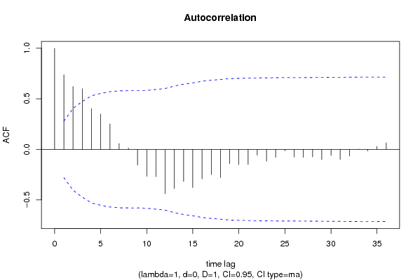
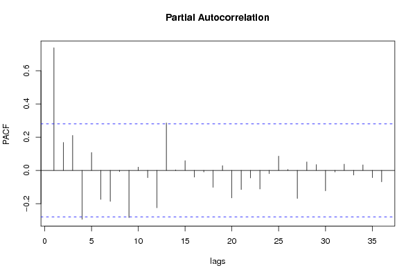
Title produced by software

(Partial) Autocorrelation Function

Date of computation

Sun, 20 Dec 2009 01:11:29 -0700

Cite this page as follows

Statistical Computations at FreeStatistics.org, Office for Research Development and Education, URL https://freestatistics.org/blog/index.php?v=date/2009/Dec/20/t1261296781ozmddkfwou9fiia.htm/, Retrieved Sat, 27 Apr 2024 11:56:09 +0000

Statistical Computations at FreeStatistics.org, Office for Research Development and Education, URL https://freestatistics.org/blog/index.php?pk=69792, Retrieved Sat, 27 Apr 2024 11:56:09 +0000

QR Codes:

Paste this QR Code to cite your computation.

Original text written by user:

IsPrivate?

No (this computation is public)

User-defined keywords

Estimated Impact

147

Family? (F = Feedback message, R = changed R code, M = changed R Module, P = changed Parameters, D = changed Data)

-     [Univariate Explorative Data Analysis] [Run Sequence gebo...] [2008-12-12 13:32:37] [76963dc1903f0f612b6153510a3818cf]
- R  D  [Univariate Explorative Data Analysis] [Run Sequence gebo...] [2008-12-17 12:14:40] [76963dc1903f0f612b6153510a3818cf]
-         [Univariate Explorative Data Analysis] [Run Sequence Plot...] [2008-12-22 18:19:51] [1ce0d16c8f4225c977b42c8fa93bc163]
- RMP       [(Partial) Autocorrelation Function] [Identifying Integ...] [2009-11-22 12:19:56] [b98453cac15ba1066b407e146608df68]
-    D        [(Partial) Autocorrelation Function] [] [2009-11-23 15:21:31] [5d885a68c2332cc44f6191ec94766bfa]
-    D            [(Partial) Autocorrelation Function] [] [2009-12-20 08:11:29] [2b679e8ec54382eeb0ec0b6bb527570a] [Current]

Feedback Forum

Post a new message

Dataseries X:

Download CSV

Histogram

Boxplots

Summary of computational transaction
Raw Input	view raw input (R code)
Raw Output	view raw output of R engine
Computing time	1 seconds
R Server	'Gwilym Jenkins' @ 72.249.127.135

\begin{tabular}{lllllllll}
\hline
Summary of computational transaction \tabularnewline
Raw Input & view raw input (R code)  \tabularnewline
Raw Output & view raw output of R engine  \tabularnewline
Computing time & 1 seconds \tabularnewline
R Server & 'Gwilym Jenkins' @ 72.249.127.135 \tabularnewline
\hline
\end{tabular}
%Source: https://freestatistics.org/blog/index.php?pk=69792&T=0

[TABLE]
[ROW][C]Summary of computational transaction[/C][/ROW]
[ROW][C]Raw Input[/C][C]view raw input (R code) [/C][/ROW]
[ROW][C]Raw Output[/C][C]view raw output of R engine [/C][/ROW]
[ROW][C]Computing time[/C][C]1 seconds[/C][/ROW]
[ROW][C]R Server[/C][C]'Gwilym Jenkins' @ 72.249.127.135[/C][/ROW]
[/TABLE]
Source: https://freestatistics.org/blog/index.php?pk=69792&T=0

Globally Unique Identifier (entire table): ba.freestatistics.org/blog/index.php?pk=69792&T=0

As an alternative you can also use a QR Code:

The GUIDs for individual cells are displayed in the table below:

Summary of computational transaction
Raw Input	view raw input (R code)
Raw Output	view raw output of R engine
Computing time	1 seconds
R Server	'Gwilym Jenkins' @ 72.249.127.135

Autocorrelation Function
Time lag k	ACF(k)	T-STAT	P-value
1	0.738476	5.1693	2e-06
2	0.621961	4.3537	3.4e-05
3	0.59945	4.1962	5.7e-05
4	0.402541	2.8178	0.003477
5	0.34937	2.4456	0.00905
6	0.250985	1.7569	0.042592
7	0.057625	0.4034	0.344213
8	0.013397	0.0938	0.462834
9	-0.155387	-1.0877	0.141023
10	-0.266899	-1.8683	0.033853
11	-0.270567	-1.894	0.03207
12	-0.439704	-3.0779	0.001705
13	-0.387417	-2.7119	0.0046
14	-0.317705	-2.2239	0.015397
15	-0.378833	-2.6518	0.005378
16	-0.292309	-2.0462	0.023063
17	-0.250297	-1.7521	0.043008
18	-0.279664	-1.9576	0.02799
19	-0.140961	-0.9867	0.164312
20	-0.151747	-1.0622	0.146669
21	-0.150325	-1.0523	0.148917
22	-0.057557	-0.4029	0.344388
23	-0.117359	-0.8215	0.207666
24	-0.078498	-0.5495	0.292585
25	-0.015678	-0.1097	0.456531
26	-0.077944	-0.5456	0.293905
27	-0.079675	-0.5577	0.289787
28	-0.075013	-0.5251	0.300944
29	-0.100674	-0.7047	0.242161
30	-0.059278	-0.4149	0.339997
31	-0.099479	-0.6964	0.244749
32	-0.066423	-0.465	0.322009
33	0.002462	0.0172	0.49316
34	-0.017264	-0.1208	0.452152
35	0.028984	0.2029	0.420031
36	0.064058	0.4484	0.327918

\begin{tabular}{lllllllll}
\hline
Autocorrelation Function \tabularnewline
Time lag k & ACF(k) & T-STAT & P-value \tabularnewline
1 & 0.738476 & 5.1693 & 2e-06 \tabularnewline
2 & 0.621961 & 4.3537 & 3.4e-05 \tabularnewline
3 & 0.59945 & 4.1962 & 5.7e-05 \tabularnewline
4 & 0.402541 & 2.8178 & 0.003477 \tabularnewline
5 & 0.34937 & 2.4456 & 0.00905 \tabularnewline
6 & 0.250985 & 1.7569 & 0.042592 \tabularnewline
7 & 0.057625 & 0.4034 & 0.344213 \tabularnewline
8 & 0.013397 & 0.0938 & 0.462834 \tabularnewline
9 & -0.155387 & -1.0877 & 0.141023 \tabularnewline
10 & -0.266899 & -1.8683 & 0.033853 \tabularnewline
11 & -0.270567 & -1.894 & 0.03207 \tabularnewline
12 & -0.439704 & -3.0779 & 0.001705 \tabularnewline
13 & -0.387417 & -2.7119 & 0.0046 \tabularnewline
14 & -0.317705 & -2.2239 & 0.015397 \tabularnewline
15 & -0.378833 & -2.6518 & 0.005378 \tabularnewline
16 & -0.292309 & -2.0462 & 0.023063 \tabularnewline
17 & -0.250297 & -1.7521 & 0.043008 \tabularnewline
18 & -0.279664 & -1.9576 & 0.02799 \tabularnewline
19 & -0.140961 & -0.9867 & 0.164312 \tabularnewline
20 & -0.151747 & -1.0622 & 0.146669 \tabularnewline
21 & -0.150325 & -1.0523 & 0.148917 \tabularnewline
22 & -0.057557 & -0.4029 & 0.344388 \tabularnewline
23 & -0.117359 & -0.8215 & 0.207666 \tabularnewline
24 & -0.078498 & -0.5495 & 0.292585 \tabularnewline
25 & -0.015678 & -0.1097 & 0.456531 \tabularnewline
26 & -0.077944 & -0.5456 & 0.293905 \tabularnewline
27 & -0.079675 & -0.5577 & 0.289787 \tabularnewline
28 & -0.075013 & -0.5251 & 0.300944 \tabularnewline
29 & -0.100674 & -0.7047 & 0.242161 \tabularnewline
30 & -0.059278 & -0.4149 & 0.339997 \tabularnewline
31 & -0.099479 & -0.6964 & 0.244749 \tabularnewline
32 & -0.066423 & -0.465 & 0.322009 \tabularnewline
33 & 0.002462 & 0.0172 & 0.49316 \tabularnewline
34 & -0.017264 & -0.1208 & 0.452152 \tabularnewline
35 & 0.028984 & 0.2029 & 0.420031 \tabularnewline
36 & 0.064058 & 0.4484 & 0.327918 \tabularnewline
\hline
\end{tabular}
%Source: https://freestatistics.org/blog/index.php?pk=69792&T=1

[TABLE]
[ROW][C]Autocorrelation Function[/C][/ROW]
[ROW][C]Time lag k[/C][C]ACF(k)[/C][C]T-STAT[/C][C]P-value[/C][/ROW]
[ROW][C]1[/C][C]0.738476[/C][C]5.1693[/C][C]2e-06[/C][/ROW]
[ROW][C]2[/C][C]0.621961[/C][C]4.3537[/C][C]3.4e-05[/C][/ROW]
[ROW][C]3[/C][C]0.59945[/C][C]4.1962[/C][C]5.7e-05[/C][/ROW]
[ROW][C]4[/C][C]0.402541[/C][C]2.8178[/C][C]0.003477[/C][/ROW]
[ROW][C]5[/C][C]0.34937[/C][C]2.4456[/C][C]0.00905[/C][/ROW]
[ROW][C]6[/C][C]0.250985[/C][C]1.7569[/C][C]0.042592[/C][/ROW]
[ROW][C]7[/C][C]0.057625[/C][C]0.4034[/C][C]0.344213[/C][/ROW]
[ROW][C]8[/C][C]0.013397[/C][C]0.0938[/C][C]0.462834[/C][/ROW]
[ROW][C]9[/C][C]-0.155387[/C][C]-1.0877[/C][C]0.141023[/C][/ROW]
[ROW][C]10[/C][C]-0.266899[/C][C]-1.8683[/C][C]0.033853[/C][/ROW]
[ROW][C]11[/C][C]-0.270567[/C][C]-1.894[/C][C]0.03207[/C][/ROW]
[ROW][C]12[/C][C]-0.439704[/C][C]-3.0779[/C][C]0.001705[/C][/ROW]
[ROW][C]13[/C][C]-0.387417[/C][C]-2.7119[/C][C]0.0046[/C][/ROW]
[ROW][C]14[/C][C]-0.317705[/C][C]-2.2239[/C][C]0.015397[/C][/ROW]
[ROW][C]15[/C][C]-0.378833[/C][C]-2.6518[/C][C]0.005378[/C][/ROW]
[ROW][C]16[/C][C]-0.292309[/C][C]-2.0462[/C][C]0.023063[/C][/ROW]
[ROW][C]17[/C][C]-0.250297[/C][C]-1.7521[/C][C]0.043008[/C][/ROW]
[ROW][C]18[/C][C]-0.279664[/C][C]-1.9576[/C][C]0.02799[/C][/ROW]
[ROW][C]19[/C][C]-0.140961[/C][C]-0.9867[/C][C]0.164312[/C][/ROW]
[ROW][C]20[/C][C]-0.151747[/C][C]-1.0622[/C][C]0.146669[/C][/ROW]
[ROW][C]21[/C][C]-0.150325[/C][C]-1.0523[/C][C]0.148917[/C][/ROW]
[ROW][C]22[/C][C]-0.057557[/C][C]-0.4029[/C][C]0.344388[/C][/ROW]
[ROW][C]23[/C][C]-0.117359[/C][C]-0.8215[/C][C]0.207666[/C][/ROW]
[ROW][C]24[/C][C]-0.078498[/C][C]-0.5495[/C][C]0.292585[/C][/ROW]
[ROW][C]25[/C][C]-0.015678[/C][C]-0.1097[/C][C]0.456531[/C][/ROW]
[ROW][C]26[/C][C]-0.077944[/C][C]-0.5456[/C][C]0.293905[/C][/ROW]
[ROW][C]27[/C][C]-0.079675[/C][C]-0.5577[/C][C]0.289787[/C][/ROW]
[ROW][C]28[/C][C]-0.075013[/C][C]-0.5251[/C][C]0.300944[/C][/ROW]
[ROW][C]29[/C][C]-0.100674[/C][C]-0.7047[/C][C]0.242161[/C][/ROW]
[ROW][C]30[/C][C]-0.059278[/C][C]-0.4149[/C][C]0.339997[/C][/ROW]
[ROW][C]31[/C][C]-0.099479[/C][C]-0.6964[/C][C]0.244749[/C][/ROW]
[ROW][C]32[/C][C]-0.066423[/C][C]-0.465[/C][C]0.322009[/C][/ROW]
[ROW][C]33[/C][C]0.002462[/C][C]0.0172[/C][C]0.49316[/C][/ROW]
[ROW][C]34[/C][C]-0.017264[/C][C]-0.1208[/C][C]0.452152[/C][/ROW]
[ROW][C]35[/C][C]0.028984[/C][C]0.2029[/C][C]0.420031[/C][/ROW]
[ROW][C]36[/C][C]0.064058[/C][C]0.4484[/C][C]0.327918[/C][/ROW]
[/TABLE]
Source: https://freestatistics.org/blog/index.php?pk=69792&T=1

Globally Unique Identifier (entire table): ba.freestatistics.org/blog/index.php?pk=69792&T=1

As an alternative you can also use a QR Code:

The GUIDs for individual cells are displayed in the table below:

Autocorrelation Function
Time lag k	ACF(k)	T-STAT	P-value
1	0.738476	5.1693	2e-06
2	0.621961	4.3537	3.4e-05
3	0.59945	4.1962	5.7e-05
4	0.402541	2.8178	0.003477
5	0.34937	2.4456	0.00905
6	0.250985	1.7569	0.042592
7	0.057625	0.4034	0.344213
8	0.013397	0.0938	0.462834
9	-0.155387	-1.0877	0.141023
10	-0.266899	-1.8683	0.033853
11	-0.270567	-1.894	0.03207
12	-0.439704	-3.0779	0.001705
13	-0.387417	-2.7119	0.0046
14	-0.317705	-2.2239	0.015397
15	-0.378833	-2.6518	0.005378
16	-0.292309	-2.0462	0.023063
17	-0.250297	-1.7521	0.043008
18	-0.279664	-1.9576	0.02799
19	-0.140961	-0.9867	0.164312
20	-0.151747	-1.0622	0.146669
21	-0.150325	-1.0523	0.148917
22	-0.057557	-0.4029	0.344388
23	-0.117359	-0.8215	0.207666
24	-0.078498	-0.5495	0.292585
25	-0.015678	-0.1097	0.456531
26	-0.077944	-0.5456	0.293905
27	-0.079675	-0.5577	0.289787
28	-0.075013	-0.5251	0.300944
29	-0.100674	-0.7047	0.242161
30	-0.059278	-0.4149	0.339997
31	-0.099479	-0.6964	0.244749
32	-0.066423	-0.465	0.322009
33	0.002462	0.0172	0.49316
34	-0.017264	-0.1208	0.452152
35	0.028984	0.2029	0.420031
36	0.064058	0.4484	0.327918

Partial Autocorrelation Function
Time lag k	PACF(k)	T-STAT	P-value
1	0.738476	5.1693	2e-06
2	0.16851	1.1796	0.121933
3	0.210765	1.4754	0.073257
4	-0.294257	-2.0598	0.022375
5	0.107717	0.754	0.227224
6	-0.174391	-1.2207	0.114014
7	-0.186535	-1.3057	0.098868
8	-0.006868	-0.0481	0.480926
9	-0.284108	-1.9888	0.026164
10	0.019805	0.1386	0.445153
11	-0.043898	-0.3073	0.379963
12	-0.224935	-1.5745	0.060899
13	0.285517	1.9986	0.025607
14	0.003186	0.0223	0.491148
15	0.058932	0.4125	0.340878
16	-0.040671	-0.2847	0.388539
17	-0.009153	-0.0641	0.474588
18	-0.101985	-0.7139	0.239339
19	0.028478	0.1993	0.421407
20	-0.165855	-1.161	0.125636
21	-0.114923	-0.8045	0.212508
22	-0.045156	-0.3161	0.376637
23	-0.111768	-0.7824	0.218879
24	-0.019816	-0.1387	0.445123
25	0.086045	0.6023	0.274871
26	0.005576	0.039	0.484513
27	-0.169016	-1.1831	0.121236
28	0.050863	0.356	0.361668
29	0.03492	0.2444	0.403957
30	-0.123121	-0.8618	0.196485
31	-0.009384	-0.0657	0.473946
32	0.037612	0.2633	0.396718
33	-0.028332	-0.1983	0.421805
34	0.033447	0.2341	0.407931
35	-0.04379	-0.3065	0.380249
36	-0.068686	-0.4808	0.316399

\begin{tabular}{lllllllll}
\hline
Partial Autocorrelation Function \tabularnewline
Time lag k & PACF(k) & T-STAT & P-value \tabularnewline
1 & 0.738476 & 5.1693 & 2e-06 \tabularnewline
2 & 0.16851 & 1.1796 & 0.121933 \tabularnewline
3 & 0.210765 & 1.4754 & 0.073257 \tabularnewline
4 & -0.294257 & -2.0598 & 0.022375 \tabularnewline
5 & 0.107717 & 0.754 & 0.227224 \tabularnewline
6 & -0.174391 & -1.2207 & 0.114014 \tabularnewline
7 & -0.186535 & -1.3057 & 0.098868 \tabularnewline
8 & -0.006868 & -0.0481 & 0.480926 \tabularnewline
9 & -0.284108 & -1.9888 & 0.026164 \tabularnewline
10 & 0.019805 & 0.1386 & 0.445153 \tabularnewline
11 & -0.043898 & -0.3073 & 0.379963 \tabularnewline
12 & -0.224935 & -1.5745 & 0.060899 \tabularnewline
13 & 0.285517 & 1.9986 & 0.025607 \tabularnewline
14 & 0.003186 & 0.0223 & 0.491148 \tabularnewline
15 & 0.058932 & 0.4125 & 0.340878 \tabularnewline
16 & -0.040671 & -0.2847 & 0.388539 \tabularnewline
17 & -0.009153 & -0.0641 & 0.474588 \tabularnewline
18 & -0.101985 & -0.7139 & 0.239339 \tabularnewline
19 & 0.028478 & 0.1993 & 0.421407 \tabularnewline
20 & -0.165855 & -1.161 & 0.125636 \tabularnewline
21 & -0.114923 & -0.8045 & 0.212508 \tabularnewline
22 & -0.045156 & -0.3161 & 0.376637 \tabularnewline
23 & -0.111768 & -0.7824 & 0.218879 \tabularnewline
24 & -0.019816 & -0.1387 & 0.445123 \tabularnewline
25 & 0.086045 & 0.6023 & 0.274871 \tabularnewline
26 & 0.005576 & 0.039 & 0.484513 \tabularnewline
27 & -0.169016 & -1.1831 & 0.121236 \tabularnewline
28 & 0.050863 & 0.356 & 0.361668 \tabularnewline
29 & 0.03492 & 0.2444 & 0.403957 \tabularnewline
30 & -0.123121 & -0.8618 & 0.196485 \tabularnewline
31 & -0.009384 & -0.0657 & 0.473946 \tabularnewline
32 & 0.037612 & 0.2633 & 0.396718 \tabularnewline
33 & -0.028332 & -0.1983 & 0.421805 \tabularnewline
34 & 0.033447 & 0.2341 & 0.407931 \tabularnewline
35 & -0.04379 & -0.3065 & 0.380249 \tabularnewline
36 & -0.068686 & -0.4808 & 0.316399 \tabularnewline
\hline
\end{tabular}
%Source: https://freestatistics.org/blog/index.php?pk=69792&T=2

[TABLE]
[ROW][C]Partial Autocorrelation Function[/C][/ROW]
[ROW][C]Time lag k[/C][C]PACF(k)[/C][C]T-STAT[/C][C]P-value[/C][/ROW]
[ROW][C]1[/C][C]0.738476[/C][C]5.1693[/C][C]2e-06[/C][/ROW]
[ROW][C]2[/C][C]0.16851[/C][C]1.1796[/C][C]0.121933[/C][/ROW]
[ROW][C]3[/C][C]0.210765[/C][C]1.4754[/C][C]0.073257[/C][/ROW]
[ROW][C]4[/C][C]-0.294257[/C][C]-2.0598[/C][C]0.022375[/C][/ROW]
[ROW][C]5[/C][C]0.107717[/C][C]0.754[/C][C]0.227224[/C][/ROW]
[ROW][C]6[/C][C]-0.174391[/C][C]-1.2207[/C][C]0.114014[/C][/ROW]
[ROW][C]7[/C][C]-0.186535[/C][C]-1.3057[/C][C]0.098868[/C][/ROW]
[ROW][C]8[/C][C]-0.006868[/C][C]-0.0481[/C][C]0.480926[/C][/ROW]
[ROW][C]9[/C][C]-0.284108[/C][C]-1.9888[/C][C]0.026164[/C][/ROW]
[ROW][C]10[/C][C]0.019805[/C][C]0.1386[/C][C]0.445153[/C][/ROW]
[ROW][C]11[/C][C]-0.043898[/C][C]-0.3073[/C][C]0.379963[/C][/ROW]
[ROW][C]12[/C][C]-0.224935[/C][C]-1.5745[/C][C]0.060899[/C][/ROW]
[ROW][C]13[/C][C]0.285517[/C][C]1.9986[/C][C]0.025607[/C][/ROW]
[ROW][C]14[/C][C]0.003186[/C][C]0.0223[/C][C]0.491148[/C][/ROW]
[ROW][C]15[/C][C]0.058932[/C][C]0.4125[/C][C]0.340878[/C][/ROW]
[ROW][C]16[/C][C]-0.040671[/C][C]-0.2847[/C][C]0.388539[/C][/ROW]
[ROW][C]17[/C][C]-0.009153[/C][C]-0.0641[/C][C]0.474588[/C][/ROW]
[ROW][C]18[/C][C]-0.101985[/C][C]-0.7139[/C][C]0.239339[/C][/ROW]
[ROW][C]19[/C][C]0.028478[/C][C]0.1993[/C][C]0.421407[/C][/ROW]
[ROW][C]20[/C][C]-0.165855[/C][C]-1.161[/C][C]0.125636[/C][/ROW]
[ROW][C]21[/C][C]-0.114923[/C][C]-0.8045[/C][C]0.212508[/C][/ROW]
[ROW][C]22[/C][C]-0.045156[/C][C]-0.3161[/C][C]0.376637[/C][/ROW]
[ROW][C]23[/C][C]-0.111768[/C][C]-0.7824[/C][C]0.218879[/C][/ROW]
[ROW][C]24[/C][C]-0.019816[/C][C]-0.1387[/C][C]0.445123[/C][/ROW]
[ROW][C]25[/C][C]0.086045[/C][C]0.6023[/C][C]0.274871[/C][/ROW]
[ROW][C]26[/C][C]0.005576[/C][C]0.039[/C][C]0.484513[/C][/ROW]
[ROW][C]27[/C][C]-0.169016[/C][C]-1.1831[/C][C]0.121236[/C][/ROW]
[ROW][C]28[/C][C]0.050863[/C][C]0.356[/C][C]0.361668[/C][/ROW]
[ROW][C]29[/C][C]0.03492[/C][C]0.2444[/C][C]0.403957[/C][/ROW]
[ROW][C]30[/C][C]-0.123121[/C][C]-0.8618[/C][C]0.196485[/C][/ROW]
[ROW][C]31[/C][C]-0.009384[/C][C]-0.0657[/C][C]0.473946[/C][/ROW]
[ROW][C]32[/C][C]0.037612[/C][C]0.2633[/C][C]0.396718[/C][/ROW]
[ROW][C]33[/C][C]-0.028332[/C][C]-0.1983[/C][C]0.421805[/C][/ROW]
[ROW][C]34[/C][C]0.033447[/C][C]0.2341[/C][C]0.407931[/C][/ROW]
[ROW][C]35[/C][C]-0.04379[/C][C]-0.3065[/C][C]0.380249[/C][/ROW]
[ROW][C]36[/C][C]-0.068686[/C][C]-0.4808[/C][C]0.316399[/C][/ROW]
[/TABLE]
Source: https://freestatistics.org/blog/index.php?pk=69792&T=2

Globally Unique Identifier (entire table): ba.freestatistics.org/blog/index.php?pk=69792&T=2

As an alternative you can also use a QR Code:

The GUIDs for individual cells are displayed in the table below:

Partial Autocorrelation Function
Time lag k	PACF(k)	T-STAT	P-value
1	0.738476	5.1693	2e-06
2	0.16851	1.1796	0.121933
3	0.210765	1.4754	0.073257
4	-0.294257	-2.0598	0.022375
5	0.107717	0.754	0.227224
6	-0.174391	-1.2207	0.114014
7	-0.186535	-1.3057	0.098868
8	-0.006868	-0.0481	0.480926
9	-0.284108	-1.9888	0.026164
10	0.019805	0.1386	0.445153
11	-0.043898	-0.3073	0.379963
12	-0.224935	-1.5745	0.060899
13	0.285517	1.9986	0.025607
14	0.003186	0.0223	0.491148
15	0.058932	0.4125	0.340878
16	-0.040671	-0.2847	0.388539
17	-0.009153	-0.0641	0.474588
18	-0.101985	-0.7139	0.239339
19	0.028478	0.1993	0.421407
20	-0.165855	-1.161	0.125636
21	-0.114923	-0.8045	0.212508
22	-0.045156	-0.3161	0.376637
23	-0.111768	-0.7824	0.218879
24	-0.019816	-0.1387	0.445123
25	0.086045	0.6023	0.274871
26	0.005576	0.039	0.484513
27	-0.169016	-1.1831	0.121236
28	0.050863	0.356	0.361668
29	0.03492	0.2444	0.403957
30	-0.123121	-0.8618	0.196485
31	-0.009384	-0.0657	0.473946
32	0.037612	0.2633	0.396718
33	-0.028332	-0.1983	0.421805
34	0.033447	0.2341	0.407931
35	-0.04379	-0.3065	0.380249
36	-0.068686	-0.4808	0.316399

Figure 1

PNG link

Postscript link

PDF link

Figure 2

PNG link

Postscript link

PDF link

Parameters (Session):

par1 = 36 ; par2 = 1 ; par3 = 0 ; par4 = 1 ; par5 = 12 ; par6 = MA ; par7 = 0.95 ;

Parameters (R input):

par1 = 36 ; par2 = 1 ; par3 = 0 ; par4 = 1 ; par5 = 12 ; par6 = MA ; par7 = 0.95 ;

R code (references can be found in the software module):

if (par1 == 'Default') {
par1 = 10*log10(length(x))
} else {
par1 <- as.numeric(par1)
}
par2 <- as.numeric(par2)
par3 <- as.numeric(par3)
par4 <- as.numeric(par4)
par5 <- as.numeric(par5)
if (par6 == 'White Noise') par6 <- 'white' else par6 <- 'ma'
par7 <- as.numeric(par7)
if (par2 == 0) {
x <- log(x)
} else {
x <- (x ^ par2 - 1) / par2
}
if (par3 > 0) x <- diff(x,lag=1,difference=par3)
if (par4 > 0) x <- diff(x,lag=par5,difference=par4)
bitmap(file='pic1.png')
racf <- acf(x, par1, main='Autocorrelation', xlab='time lag', ylab='ACF', ci.type=par6, ci=par7, sub=paste('(lambda=',par2,', d=',par3,', D=',par4,', CI=', par7, ', CI type=',par6,')',sep=''))
dev.off()
bitmap(file='pic2.png')
rpacf <- pacf(x,par1,main='Partial Autocorrelation',xlab='lags',ylab='PACF')
dev.off()
(myacf <- c(racf$acf))
(mypacf <- c(rpacf$acf))
lengthx <- length(x)
sqrtn <- sqrt(lengthx)
load(file='createtable')
a<-table.start()
a<-table.row.start(a)
a<-table.element(a,'Autocorrelation Function',4,TRUE)
a<-table.row.end(a)
a<-table.row.start(a)
a<-table.element(a,'Time lag k',header=TRUE)
a<-table.element(a,hyperlink('basics.htm','ACF(k)','click here for more information about the Autocorrelation Function'),header=TRUE)
a<-table.element(a,'T-STAT',header=TRUE)
a<-table.element(a,'P-value',header=TRUE)
a<-table.row.end(a)
for (i in 2:(par1+1)) {
a<-table.row.start(a)
a<-table.element(a,i-1,header=TRUE)
a<-table.element(a,round(myacf[i],6))
mytstat <- myacf[i]*sqrtn
a<-table.element(a,round(mytstat,4))
a<-table.element(a,round(1-pt(abs(mytstat),lengthx),6))
a<-table.row.end(a)
}
a<-table.end(a)
table.save(a,file='mytable.tab')
a<-table.start()
a<-table.row.start(a)
a<-table.element(a,'Partial Autocorrelation Function',4,TRUE)
a<-table.row.end(a)
a<-table.row.start(a)
a<-table.element(a,'Time lag k',header=TRUE)
a<-table.element(a,hyperlink('basics.htm','PACF(k)','click here for more information about the Partial Autocorrelation Function'),header=TRUE)
a<-table.element(a,'T-STAT',header=TRUE)
a<-table.element(a,'P-value',header=TRUE)
a<-table.row.end(a)
for (i in 1:par1) {
a<-table.row.start(a)
a<-table.element(a,i,header=TRUE)
a<-table.element(a,round(mypacf[i],6))
mytstat <- mypacf[i]*sqrtn
a<-table.element(a,round(mytstat,4))
a<-table.element(a,round(1-pt(abs(mytstat),lengthx),6))
a<-table.row.end(a)
}
a<-table.end(a)
table.save(a,file='mytable1.tab')

Free Statistics

Description of Statistical Computation

Tree of Dependent Computations

Dataset

Tables (Output of Computation)

Figures (Output of Computation)

Input Parameters & R Code