Repository of Reproducible Computations

Free Statistics

of Irreproducible Research!

Author's title

Author

*The author of this computation has been verified*

R Software Module

rwasp_autocorrelation.wasp

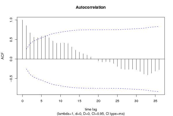
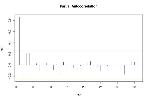
Title produced by software

(Partial) Autocorrelation Function

Date of computation

Sun, 20 Dec 2009 04:19:07 -0700

Cite this page as follows

Statistical Computations at FreeStatistics.org, Office for Research Development and Education, URL https://freestatistics.org/blog/index.php?v=date/2009/Dec/20/t1261308011ecoav0nfkloinuy.htm/, Retrieved Sat, 27 Apr 2024 09:24:42 +0000

Statistical Computations at FreeStatistics.org, Office for Research Development and Education, URL https://freestatistics.org/blog/index.php?pk=69840, Retrieved Sat, 27 Apr 2024 09:24:42 +0000

QR Codes:

Paste this QR Code to cite your computation.

Original text written by user:

IsPrivate?

No (this computation is public)

User-defined keywords

Estimated Impact

141

Family? (F = Feedback message, R = changed R code, M = changed R Module, P = changed Parameters, D = changed Data)

-     [Univariate Explorative Data Analysis] [Run Sequence gebo...] [2008-12-12 13:32:37] [76963dc1903f0f612b6153510a3818cf]
- R  D  [Univariate Explorative Data Analysis] [Run Sequence gebo...] [2008-12-17 12:14:40] [76963dc1903f0f612b6153510a3818cf]
-         [Univariate Explorative Data Analysis] [Run Sequence Plot...] [2008-12-22 18:19:51] [1ce0d16c8f4225c977b42c8fa93bc163]
- RMP       [(Partial) Autocorrelation Function] [Identifying Integ...] [2009-11-22 12:16:10] [b98453cac15ba1066b407e146608df68]
-    D        [(Partial) Autocorrelation Function] [ws8] [2009-11-24 20:12:27] [8b1aef4e7013bd33fbc2a5833375c5f5]
-    D          [(Partial) Autocorrelation Function] [WS8(1)] [2009-11-27 10:20:58] [7d268329e554b8694908ba13e6e6f258]
-    D              [(Partial) Autocorrelation Function] [] [2009-12-20 11:19:07] [4d89445a8ea4b299af2ee123046cffa6] [Current]

Feedback Forum

Post a new message

Dataseries X:

Download CSV

Histogram

Boxplots

10.9
10
9.2
9.2
9.5
9.6
9.5
9.1
8.9
9
10.1
10.3
10.2
9.6
9.2
9.3
9.4
9.4
9.2
9
9
9
9.8
10
9.8
9.3
9
9
9.1
9.1
9.1
9.2
8.8
8.3
8.4
8.1
7.7
7.9
7.9
8
7.9
7.6
7.1
6.8
6.5
6.9
8.2
8.7
8.3
7.9
7.5
7.8
8.3
8.4
8.2
7.7
7.2
7.3
8.1
8.5

Summary of computational transaction
Raw Input	view raw input (R code)
Raw Output	view raw output of R engine
Computing time	1 seconds
R Server	'Gwilym Jenkins' @ 72.249.127.135

\begin{tabular}{lllllllll}
\hline
Summary of computational transaction \tabularnewline
Raw Input & view raw input (R code)  \tabularnewline
Raw Output & view raw output of R engine  \tabularnewline
Computing time & 1 seconds \tabularnewline
R Server & 'Gwilym Jenkins' @ 72.249.127.135 \tabularnewline
\hline
\end{tabular}
%Source: https://freestatistics.org/blog/index.php?pk=69840&T=0

[TABLE]
[ROW][C]Summary of computational transaction[/C][/ROW]
[ROW][C]Raw Input[/C][C]view raw input (R code) [/C][/ROW]
[ROW][C]Raw Output[/C][C]view raw output of R engine [/C][/ROW]
[ROW][C]Computing time[/C][C]1 seconds[/C][/ROW]
[ROW][C]R Server[/C][C]'Gwilym Jenkins' @ 72.249.127.135[/C][/ROW]
[/TABLE]
Source: https://freestatistics.org/blog/index.php?pk=69840&T=0

Globally Unique Identifier (entire table): ba.freestatistics.org/blog/index.php?pk=69840&T=0

As an alternative you can also use a QR Code:

The GUIDs for individual cells are displayed in the table below:

Summary of computational transaction
Raw Input	view raw input (R code)
Raw Output	view raw output of R engine
Computing time	1 seconds
R Server	'Gwilym Jenkins' @ 72.249.127.135

Autocorrelation Function
Time lag k	ACF(k)	T-STAT	P-value
1	0.858187	6.6475	0
2	0.6716	5.2022	1e-06
3	0.560884	4.3446	2.7e-05
4	0.545335	4.2241	4.1e-05
5	0.583365	4.5187	1.5e-05
6	0.600225	4.6493	9e-06
7	0.547021	4.2372	4e-05
8	0.462158	3.5799	0.000344
9	0.406519	3.1489	0.001277
10	0.408205	3.1619	0.001229
11	0.411577	3.1881	0.001138
12	0.395279	3.0618	0.001645
13	0.311353	2.4117	0.009477
14	0.228925	1.7732	0.040632
15	0.176845	1.3698	0.087921
16	0.136006	1.0535	0.148168
17	0.101161	0.7836	0.218181
18	0.054327	0.4208	0.337695
19	-0.001873	-0.0145	0.494235
20	-0.052267	-0.4049	0.343511
21	-0.07662	-0.5935	0.277539
22	-0.066317	-0.5137	0.304678
23	-0.074185	-0.5746	0.283843
24	-0.114088	-0.8837	0.190188
25	-0.190895	-1.4787	0.07223
26	-0.249906	-1.9358	0.028806
27	-0.267891	-2.0751	0.021138
28	-0.26583	-2.0591	0.021916
29	-0.26021	-2.0156	0.024165
30	-0.274447	-2.1259	0.01882
31	-0.319595	-2.4756	0.008071
32	-0.386474	-2.9936	0.002
33	-0.408393	-3.1634	0.001224
34	-0.363994	-2.8195	0.003254
35	-0.310229	-2.403	0.009685
36	-0.274073	-2.123	0.018946

\begin{tabular}{lllllllll}
\hline
Autocorrelation Function \tabularnewline
Time lag k & ACF(k) & T-STAT & P-value \tabularnewline
1 & 0.858187 & 6.6475 & 0 \tabularnewline
2 & 0.6716 & 5.2022 & 1e-06 \tabularnewline
3 & 0.560884 & 4.3446 & 2.7e-05 \tabularnewline
4 & 0.545335 & 4.2241 & 4.1e-05 \tabularnewline
5 & 0.583365 & 4.5187 & 1.5e-05 \tabularnewline
6 & 0.600225 & 4.6493 & 9e-06 \tabularnewline
7 & 0.547021 & 4.2372 & 4e-05 \tabularnewline
8 & 0.462158 & 3.5799 & 0.000344 \tabularnewline
9 & 0.406519 & 3.1489 & 0.001277 \tabularnewline
10 & 0.408205 & 3.1619 & 0.001229 \tabularnewline
11 & 0.411577 & 3.1881 & 0.001138 \tabularnewline
12 & 0.395279 & 3.0618 & 0.001645 \tabularnewline
13 & 0.311353 & 2.4117 & 0.009477 \tabularnewline
14 & 0.228925 & 1.7732 & 0.040632 \tabularnewline
15 & 0.176845 & 1.3698 & 0.087921 \tabularnewline
16 & 0.136006 & 1.0535 & 0.148168 \tabularnewline
17 & 0.101161 & 0.7836 & 0.218181 \tabularnewline
18 & 0.054327 & 0.4208 & 0.337695 \tabularnewline
19 & -0.001873 & -0.0145 & 0.494235 \tabularnewline
20 & -0.052267 & -0.4049 & 0.343511 \tabularnewline
21 & -0.07662 & -0.5935 & 0.277539 \tabularnewline
22 & -0.066317 & -0.5137 & 0.304678 \tabularnewline
23 & -0.074185 & -0.5746 & 0.283843 \tabularnewline
24 & -0.114088 & -0.8837 & 0.190188 \tabularnewline
25 & -0.190895 & -1.4787 & 0.07223 \tabularnewline
26 & -0.249906 & -1.9358 & 0.028806 \tabularnewline
27 & -0.267891 & -2.0751 & 0.021138 \tabularnewline
28 & -0.26583 & -2.0591 & 0.021916 \tabularnewline
29 & -0.26021 & -2.0156 & 0.024165 \tabularnewline
30 & -0.274447 & -2.1259 & 0.01882 \tabularnewline
31 & -0.319595 & -2.4756 & 0.008071 \tabularnewline
32 & -0.386474 & -2.9936 & 0.002 \tabularnewline
33 & -0.408393 & -3.1634 & 0.001224 \tabularnewline
34 & -0.363994 & -2.8195 & 0.003254 \tabularnewline
35 & -0.310229 & -2.403 & 0.009685 \tabularnewline
36 & -0.274073 & -2.123 & 0.018946 \tabularnewline
\hline
\end{tabular}
%Source: https://freestatistics.org/blog/index.php?pk=69840&T=1

[TABLE]
[ROW][C]Autocorrelation Function[/C][/ROW]
[ROW][C]Time lag k[/C][C]ACF(k)[/C][C]T-STAT[/C][C]P-value[/C][/ROW]
[ROW][C]1[/C][C]0.858187[/C][C]6.6475[/C][C]0[/C][/ROW]
[ROW][C]2[/C][C]0.6716[/C][C]5.2022[/C][C]1e-06[/C][/ROW]
[ROW][C]3[/C][C]0.560884[/C][C]4.3446[/C][C]2.7e-05[/C][/ROW]
[ROW][C]4[/C][C]0.545335[/C][C]4.2241[/C][C]4.1e-05[/C][/ROW]
[ROW][C]5[/C][C]0.583365[/C][C]4.5187[/C][C]1.5e-05[/C][/ROW]
[ROW][C]6[/C][C]0.600225[/C][C]4.6493[/C][C]9e-06[/C][/ROW]
[ROW][C]7[/C][C]0.547021[/C][C]4.2372[/C][C]4e-05[/C][/ROW]
[ROW][C]8[/C][C]0.462158[/C][C]3.5799[/C][C]0.000344[/C][/ROW]
[ROW][C]9[/C][C]0.406519[/C][C]3.1489[/C][C]0.001277[/C][/ROW]
[ROW][C]10[/C][C]0.408205[/C][C]3.1619[/C][C]0.001229[/C][/ROW]
[ROW][C]11[/C][C]0.411577[/C][C]3.1881[/C][C]0.001138[/C][/ROW]
[ROW][C]12[/C][C]0.395279[/C][C]3.0618[/C][C]0.001645[/C][/ROW]
[ROW][C]13[/C][C]0.311353[/C][C]2.4117[/C][C]0.009477[/C][/ROW]
[ROW][C]14[/C][C]0.228925[/C][C]1.7732[/C][C]0.040632[/C][/ROW]
[ROW][C]15[/C][C]0.176845[/C][C]1.3698[/C][C]0.087921[/C][/ROW]
[ROW][C]16[/C][C]0.136006[/C][C]1.0535[/C][C]0.148168[/C][/ROW]
[ROW][C]17[/C][C]0.101161[/C][C]0.7836[/C][C]0.218181[/C][/ROW]
[ROW][C]18[/C][C]0.054327[/C][C]0.4208[/C][C]0.337695[/C][/ROW]
[ROW][C]19[/C][C]-0.001873[/C][C]-0.0145[/C][C]0.494235[/C][/ROW]
[ROW][C]20[/C][C]-0.052267[/C][C]-0.4049[/C][C]0.343511[/C][/ROW]
[ROW][C]21[/C][C]-0.07662[/C][C]-0.5935[/C][C]0.277539[/C][/ROW]
[ROW][C]22[/C][C]-0.066317[/C][C]-0.5137[/C][C]0.304678[/C][/ROW]
[ROW][C]23[/C][C]-0.074185[/C][C]-0.5746[/C][C]0.283843[/C][/ROW]
[ROW][C]24[/C][C]-0.114088[/C][C]-0.8837[/C][C]0.190188[/C][/ROW]
[ROW][C]25[/C][C]-0.190895[/C][C]-1.4787[/C][C]0.07223[/C][/ROW]
[ROW][C]26[/C][C]-0.249906[/C][C]-1.9358[/C][C]0.028806[/C][/ROW]
[ROW][C]27[/C][C]-0.267891[/C][C]-2.0751[/C][C]0.021138[/C][/ROW]
[ROW][C]28[/C][C]-0.26583[/C][C]-2.0591[/C][C]0.021916[/C][/ROW]
[ROW][C]29[/C][C]-0.26021[/C][C]-2.0156[/C][C]0.024165[/C][/ROW]
[ROW][C]30[/C][C]-0.274447[/C][C]-2.1259[/C][C]0.01882[/C][/ROW]
[ROW][C]31[/C][C]-0.319595[/C][C]-2.4756[/C][C]0.008071[/C][/ROW]
[ROW][C]32[/C][C]-0.386474[/C][C]-2.9936[/C][C]0.002[/C][/ROW]
[ROW][C]33[/C][C]-0.408393[/C][C]-3.1634[/C][C]0.001224[/C][/ROW]
[ROW][C]34[/C][C]-0.363994[/C][C]-2.8195[/C][C]0.003254[/C][/ROW]
[ROW][C]35[/C][C]-0.310229[/C][C]-2.403[/C][C]0.009685[/C][/ROW]
[ROW][C]36[/C][C]-0.274073[/C][C]-2.123[/C][C]0.018946[/C][/ROW]
[/TABLE]
Source: https://freestatistics.org/blog/index.php?pk=69840&T=1

Globally Unique Identifier (entire table): ba.freestatistics.org/blog/index.php?pk=69840&T=1

As an alternative you can also use a QR Code:

The GUIDs for individual cells are displayed in the table below:

Autocorrelation Function
Time lag k	ACF(k)	T-STAT	P-value
1	0.858187	6.6475	0
2	0.6716	5.2022	1e-06
3	0.560884	4.3446	2.7e-05
4	0.545335	4.2241	4.1e-05
5	0.583365	4.5187	1.5e-05
6	0.600225	4.6493	9e-06
7	0.547021	4.2372	4e-05
8	0.462158	3.5799	0.000344
9	0.406519	3.1489	0.001277
10	0.408205	3.1619	0.001229
11	0.411577	3.1881	0.001138
12	0.395279	3.0618	0.001645
13	0.311353	2.4117	0.009477
14	0.228925	1.7732	0.040632
15	0.176845	1.3698	0.087921
16	0.136006	1.0535	0.148168
17	0.101161	0.7836	0.218181
18	0.054327	0.4208	0.337695
19	-0.001873	-0.0145	0.494235
20	-0.052267	-0.4049	0.343511
21	-0.07662	-0.5935	0.277539
22	-0.066317	-0.5137	0.304678
23	-0.074185	-0.5746	0.283843
24	-0.114088	-0.8837	0.190188
25	-0.190895	-1.4787	0.07223
26	-0.249906	-1.9358	0.028806
27	-0.267891	-2.0751	0.021138
28	-0.26583	-2.0591	0.021916
29	-0.26021	-2.0156	0.024165
30	-0.274447	-2.1259	0.01882
31	-0.319595	-2.4756	0.008071
32	-0.386474	-2.9936	0.002
33	-0.408393	-3.1634	0.001224
34	-0.363994	-2.8195	0.003254
35	-0.310229	-2.403	0.009685
36	-0.274073	-2.123	0.018946

Partial Autocorrelation Function
Time lag k	PACF(k)	T-STAT	P-value
1	0.858187	6.6475	0
2	-0.246226	-1.9073	0.030639
3	0.217823	1.6872	0.048374
4	0.213234	1.6517	0.05191
5	0.174284	1.35	0.091044
6	0.026991	0.2091	0.417549
7	-0.094942	-0.7354	0.232475
8	-0.011933	-0.0924	0.463333
9	0.041265	0.3196	0.375176
10	0.077511	0.6004	0.27525
11	-0.08848	-0.6854	0.247878
12	0.010857	0.0841	0.466629
13	-0.214268	-1.6597	0.051095
14	0.052886	0.4097	0.341758
15	-0.085962	-0.6659	0.254027
16	-0.142488	-1.1037	0.137064
17	-0.048433	-0.3752	0.354432
18	-0.084499	-0.6545	0.257636
19	-0.015498	-0.12	0.452423
20	-0.064558	-0.5001	0.30943
21	0.031149	0.2413	0.405081
22	0.064988	0.5034	0.308264
23	-0.030697	-0.2378	0.406431
24	-0.051606	-0.3997	0.345383
25	-0.106713	-0.8266	0.205871
26	0.027482	0.2129	0.416073
27	-0.018797	-0.1456	0.442361
28	-0.011587	-0.0898	0.464391
29	0.001176	0.0091	0.496383
30	-0.001886	-0.0146	0.494197
31	-0.065293	-0.5058	0.307441
32	-0.167166	-1.2949	0.100164
33	0.079859	0.6186	0.269265
34	0.063933	0.4952	0.311126
35	0.049074	0.3801	0.352597
36	0.061399	0.4756	0.318045

\begin{tabular}{lllllllll}
\hline
Partial Autocorrelation Function \tabularnewline
Time lag k & PACF(k) & T-STAT & P-value \tabularnewline
1 & 0.858187 & 6.6475 & 0 \tabularnewline
2 & -0.246226 & -1.9073 & 0.030639 \tabularnewline
3 & 0.217823 & 1.6872 & 0.048374 \tabularnewline
4 & 0.213234 & 1.6517 & 0.05191 \tabularnewline
5 & 0.174284 & 1.35 & 0.091044 \tabularnewline
6 & 0.026991 & 0.2091 & 0.417549 \tabularnewline
7 & -0.094942 & -0.7354 & 0.232475 \tabularnewline
8 & -0.011933 & -0.0924 & 0.463333 \tabularnewline
9 & 0.041265 & 0.3196 & 0.375176 \tabularnewline
10 & 0.077511 & 0.6004 & 0.27525 \tabularnewline
11 & -0.08848 & -0.6854 & 0.247878 \tabularnewline
12 & 0.010857 & 0.0841 & 0.466629 \tabularnewline
13 & -0.214268 & -1.6597 & 0.051095 \tabularnewline
14 & 0.052886 & 0.4097 & 0.341758 \tabularnewline
15 & -0.085962 & -0.6659 & 0.254027 \tabularnewline
16 & -0.142488 & -1.1037 & 0.137064 \tabularnewline
17 & -0.048433 & -0.3752 & 0.354432 \tabularnewline
18 & -0.084499 & -0.6545 & 0.257636 \tabularnewline
19 & -0.015498 & -0.12 & 0.452423 \tabularnewline
20 & -0.064558 & -0.5001 & 0.30943 \tabularnewline
21 & 0.031149 & 0.2413 & 0.405081 \tabularnewline
22 & 0.064988 & 0.5034 & 0.308264 \tabularnewline
23 & -0.030697 & -0.2378 & 0.406431 \tabularnewline
24 & -0.051606 & -0.3997 & 0.345383 \tabularnewline
25 & -0.106713 & -0.8266 & 0.205871 \tabularnewline
26 & 0.027482 & 0.2129 & 0.416073 \tabularnewline
27 & -0.018797 & -0.1456 & 0.442361 \tabularnewline
28 & -0.011587 & -0.0898 & 0.464391 \tabularnewline
29 & 0.001176 & 0.0091 & 0.496383 \tabularnewline
30 & -0.001886 & -0.0146 & 0.494197 \tabularnewline
31 & -0.065293 & -0.5058 & 0.307441 \tabularnewline
32 & -0.167166 & -1.2949 & 0.100164 \tabularnewline
33 & 0.079859 & 0.6186 & 0.269265 \tabularnewline
34 & 0.063933 & 0.4952 & 0.311126 \tabularnewline
35 & 0.049074 & 0.3801 & 0.352597 \tabularnewline
36 & 0.061399 & 0.4756 & 0.318045 \tabularnewline
\hline
\end{tabular}
%Source: https://freestatistics.org/blog/index.php?pk=69840&T=2

[TABLE]
[ROW][C]Partial Autocorrelation Function[/C][/ROW]
[ROW][C]Time lag k[/C][C]PACF(k)[/C][C]T-STAT[/C][C]P-value[/C][/ROW]
[ROW][C]1[/C][C]0.858187[/C][C]6.6475[/C][C]0[/C][/ROW]
[ROW][C]2[/C][C]-0.246226[/C][C]-1.9073[/C][C]0.030639[/C][/ROW]
[ROW][C]3[/C][C]0.217823[/C][C]1.6872[/C][C]0.048374[/C][/ROW]
[ROW][C]4[/C][C]0.213234[/C][C]1.6517[/C][C]0.05191[/C][/ROW]
[ROW][C]5[/C][C]0.174284[/C][C]1.35[/C][C]0.091044[/C][/ROW]
[ROW][C]6[/C][C]0.026991[/C][C]0.2091[/C][C]0.417549[/C][/ROW]
[ROW][C]7[/C][C]-0.094942[/C][C]-0.7354[/C][C]0.232475[/C][/ROW]
[ROW][C]8[/C][C]-0.011933[/C][C]-0.0924[/C][C]0.463333[/C][/ROW]
[ROW][C]9[/C][C]0.041265[/C][C]0.3196[/C][C]0.375176[/C][/ROW]
[ROW][C]10[/C][C]0.077511[/C][C]0.6004[/C][C]0.27525[/C][/ROW]
[ROW][C]11[/C][C]-0.08848[/C][C]-0.6854[/C][C]0.247878[/C][/ROW]
[ROW][C]12[/C][C]0.010857[/C][C]0.0841[/C][C]0.466629[/C][/ROW]
[ROW][C]13[/C][C]-0.214268[/C][C]-1.6597[/C][C]0.051095[/C][/ROW]
[ROW][C]14[/C][C]0.052886[/C][C]0.4097[/C][C]0.341758[/C][/ROW]
[ROW][C]15[/C][C]-0.085962[/C][C]-0.6659[/C][C]0.254027[/C][/ROW]
[ROW][C]16[/C][C]-0.142488[/C][C]-1.1037[/C][C]0.137064[/C][/ROW]
[ROW][C]17[/C][C]-0.048433[/C][C]-0.3752[/C][C]0.354432[/C][/ROW]
[ROW][C]18[/C][C]-0.084499[/C][C]-0.6545[/C][C]0.257636[/C][/ROW]
[ROW][C]19[/C][C]-0.015498[/C][C]-0.12[/C][C]0.452423[/C][/ROW]
[ROW][C]20[/C][C]-0.064558[/C][C]-0.5001[/C][C]0.30943[/C][/ROW]
[ROW][C]21[/C][C]0.031149[/C][C]0.2413[/C][C]0.405081[/C][/ROW]
[ROW][C]22[/C][C]0.064988[/C][C]0.5034[/C][C]0.308264[/C][/ROW]
[ROW][C]23[/C][C]-0.030697[/C][C]-0.2378[/C][C]0.406431[/C][/ROW]
[ROW][C]24[/C][C]-0.051606[/C][C]-0.3997[/C][C]0.345383[/C][/ROW]
[ROW][C]25[/C][C]-0.106713[/C][C]-0.8266[/C][C]0.205871[/C][/ROW]
[ROW][C]26[/C][C]0.027482[/C][C]0.2129[/C][C]0.416073[/C][/ROW]
[ROW][C]27[/C][C]-0.018797[/C][C]-0.1456[/C][C]0.442361[/C][/ROW]
[ROW][C]28[/C][C]-0.011587[/C][C]-0.0898[/C][C]0.464391[/C][/ROW]
[ROW][C]29[/C][C]0.001176[/C][C]0.0091[/C][C]0.496383[/C][/ROW]
[ROW][C]30[/C][C]-0.001886[/C][C]-0.0146[/C][C]0.494197[/C][/ROW]
[ROW][C]31[/C][C]-0.065293[/C][C]-0.5058[/C][C]0.307441[/C][/ROW]
[ROW][C]32[/C][C]-0.167166[/C][C]-1.2949[/C][C]0.100164[/C][/ROW]
[ROW][C]33[/C][C]0.079859[/C][C]0.6186[/C][C]0.269265[/C][/ROW]
[ROW][C]34[/C][C]0.063933[/C][C]0.4952[/C][C]0.311126[/C][/ROW]
[ROW][C]35[/C][C]0.049074[/C][C]0.3801[/C][C]0.352597[/C][/ROW]
[ROW][C]36[/C][C]0.061399[/C][C]0.4756[/C][C]0.318045[/C][/ROW]
[/TABLE]
Source: https://freestatistics.org/blog/index.php?pk=69840&T=2

Globally Unique Identifier (entire table): ba.freestatistics.org/blog/index.php?pk=69840&T=2

As an alternative you can also use a QR Code:

The GUIDs for individual cells are displayed in the table below:

Partial Autocorrelation Function
Time lag k	PACF(k)	T-STAT	P-value
1	0.858187	6.6475	0
2	-0.246226	-1.9073	0.030639
3	0.217823	1.6872	0.048374
4	0.213234	1.6517	0.05191
5	0.174284	1.35	0.091044
6	0.026991	0.2091	0.417549
7	-0.094942	-0.7354	0.232475
8	-0.011933	-0.0924	0.463333
9	0.041265	0.3196	0.375176
10	0.077511	0.6004	0.27525
11	-0.08848	-0.6854	0.247878
12	0.010857	0.0841	0.466629
13	-0.214268	-1.6597	0.051095
14	0.052886	0.4097	0.341758
15	-0.085962	-0.6659	0.254027
16	-0.142488	-1.1037	0.137064
17	-0.048433	-0.3752	0.354432
18	-0.084499	-0.6545	0.257636
19	-0.015498	-0.12	0.452423
20	-0.064558	-0.5001	0.30943
21	0.031149	0.2413	0.405081
22	0.064988	0.5034	0.308264
23	-0.030697	-0.2378	0.406431
24	-0.051606	-0.3997	0.345383
25	-0.106713	-0.8266	0.205871
26	0.027482	0.2129	0.416073
27	-0.018797	-0.1456	0.442361
28	-0.011587	-0.0898	0.464391
29	0.001176	0.0091	0.496383
30	-0.001886	-0.0146	0.494197
31	-0.065293	-0.5058	0.307441
32	-0.167166	-1.2949	0.100164
33	0.079859	0.6186	0.269265
34	0.063933	0.4952	0.311126
35	0.049074	0.3801	0.352597
36	0.061399	0.4756	0.318045

Figure 1

PNG link

Postscript link

PDF link

Figure 2

PNG link

Postscript link

PDF link

Parameters (Session):

par1 = 36 ; par2 = 1 ; par3 = 0 ; par4 = 0 ; par5 = 12 ; par6 = MA ; par7 = 0.95 ;

Parameters (R input):

par1 = 36 ; par2 = 1 ; par3 = 0 ; par4 = 0 ; par5 = 12 ; par6 = MA ; par7 = 0.95 ;

R code (references can be found in the software module):

if (par1 == 'Default') {
par1 = 10*log10(length(x))
} else {
par1 <- as.numeric(par1)
}
par2 <- as.numeric(par2)
par3 <- as.numeric(par3)
par4 <- as.numeric(par4)
par5 <- as.numeric(par5)
if (par6 == 'White Noise') par6 <- 'white' else par6 <- 'ma'
par7 <- as.numeric(par7)
if (par2 == 0) {
x <- log(x)
} else {
x <- (x ^ par2 - 1) / par2
}
if (par3 > 0) x <- diff(x,lag=1,difference=par3)
if (par4 > 0) x <- diff(x,lag=par5,difference=par4)
bitmap(file='pic1.png')
racf <- acf(x, par1, main='Autocorrelation', xlab='time lag', ylab='ACF', ci.type=par6, ci=par7, sub=paste('(lambda=',par2,', d=',par3,', D=',par4,', CI=', par7, ', CI type=',par6,')',sep=''))
dev.off()
bitmap(file='pic2.png')
rpacf <- pacf(x,par1,main='Partial Autocorrelation',xlab='lags',ylab='PACF')
dev.off()
(myacf <- c(racf$acf))
(mypacf <- c(rpacf$acf))
lengthx <- length(x)
sqrtn <- sqrt(lengthx)
load(file='createtable')
a<-table.start()
a<-table.row.start(a)
a<-table.element(a,'Autocorrelation Function',4,TRUE)
a<-table.row.end(a)
a<-table.row.start(a)
a<-table.element(a,'Time lag k',header=TRUE)
a<-table.element(a,hyperlink('basics.htm','ACF(k)','click here for more information about the Autocorrelation Function'),header=TRUE)
a<-table.element(a,'T-STAT',header=TRUE)
a<-table.element(a,'P-value',header=TRUE)
a<-table.row.end(a)
for (i in 2:(par1+1)) {
a<-table.row.start(a)
a<-table.element(a,i-1,header=TRUE)
a<-table.element(a,round(myacf[i],6))
mytstat <- myacf[i]*sqrtn
a<-table.element(a,round(mytstat,4))
a<-table.element(a,round(1-pt(abs(mytstat),lengthx),6))
a<-table.row.end(a)
}
a<-table.end(a)
table.save(a,file='mytable.tab')
a<-table.start()
a<-table.row.start(a)
a<-table.element(a,'Partial Autocorrelation Function',4,TRUE)
a<-table.row.end(a)
a<-table.row.start(a)
a<-table.element(a,'Time lag k',header=TRUE)
a<-table.element(a,hyperlink('basics.htm','PACF(k)','click here for more information about the Partial Autocorrelation Function'),header=TRUE)
a<-table.element(a,'T-STAT',header=TRUE)
a<-table.element(a,'P-value',header=TRUE)
a<-table.row.end(a)
for (i in 1:par1) {
a<-table.row.start(a)
a<-table.element(a,i,header=TRUE)
a<-table.element(a,round(mypacf[i],6))
mytstat <- mypacf[i]*sqrtn
a<-table.element(a,round(mytstat,4))
a<-table.element(a,round(1-pt(abs(mytstat),lengthx),6))
a<-table.row.end(a)
}
a<-table.end(a)
table.save(a,file='mytable1.tab')

Free Statistics

Description of Statistical Computation

Tree of Dependent Computations

Dataset

Tables (Output of Computation)

Figures (Output of Computation)

Input Parameters & R Code