Free Statistics
of Irreproducible Research!
Description of Statistical Computation | |||||||||||||||||||||
|---|---|---|---|---|---|---|---|---|---|---|---|---|---|---|---|---|---|---|---|---|---|
| Author's title | |||||||||||||||||||||
| Author | *The author of this computation has been verified* | ||||||||||||||||||||
| R Software Module | rwasp_cloud.wasp | ||||||||||||||||||||
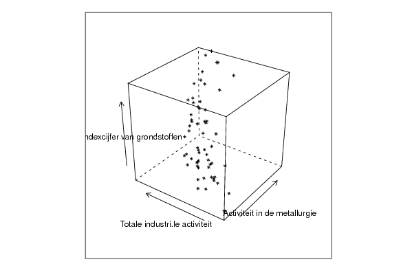
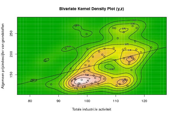
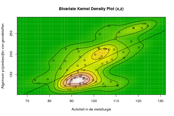
| Title produced by software | Trivariate Scatterplots | ||||||||||||||||||||
| Date of computation | Tue, 22 Dec 2009 10:37:24 -0700 | ||||||||||||||||||||
| Cite this page as follows | Statistical Computations at FreeStatistics.org, Office for Research Development and Education, URL https://freestatistics.org/blog/index.php?v=date/2009/Dec/22/t12615035345r9cxyuncrpur80.htm/, Retrieved Sat, 04 May 2024 14:59:25 +0000 | ||||||||||||||||||||
| Statistical Computations at FreeStatistics.org, Office for Research Development and Education, URL https://freestatistics.org/blog/index.php?pk=70464, Retrieved Sat, 04 May 2024 14:59:25 +0000 | |||||||||||||||||||||
| QR Codes: | |||||||||||||||||||||
|
| |||||||||||||||||||||
| Original text written by user: | |||||||||||||||||||||
| IsPrivate? | No (this computation is public) | ||||||||||||||||||||
| User-defined keywords | |||||||||||||||||||||
| Estimated Impact | 172 | ||||||||||||||||||||
Tree of Dependent Computations | |||||||||||||||||||||
| Family? (F = Feedback message, R = changed R code, M = changed R Module, P = changed Parameters, D = changed Data) | |||||||||||||||||||||
| - [Bivariate Data Series] [Bivariate dataset] [2008-01-05 23:51:08] [74be16979710d4c4e7c6647856088456] - PD [Bivariate Data Series] [Reproduction Part 1] [2009-10-26 18:51:43] [96e597a9107bfe8c07649cce3d4f6fec] - RMPD [Bivariate Explorative Data Analysis] [JJ Workshop 4, De...] [2009-10-26 19:42:48] [96e597a9107bfe8c07649cce3d4f6fec] - D [Bivariate Explorative Data Analysis] [JJ Workshop 4, de...] [2009-10-27 18:56:34] [96e597a9107bfe8c07649cce3d4f6fec] - RM D [Bivariate Explorative Data Analysis] [JJ Workshop 5, mo...] [2009-11-02 13:09:27] [96e597a9107bfe8c07649cce3d4f6fec] - RMPD [Trivariate Scatterplots] [JJ Workshop 5, mo...] [2009-11-02 13:45:08] [96e597a9107bfe8c07649cce3d4f6fec] - PD [Trivariate Scatterplots] [JJ Workshop 5, mo...] [2009-11-02 15:07:04] [96e597a9107bfe8c07649cce3d4f6fec] - PD [Trivariate Scatterplots] [Paper, Trivariate...] [2009-12-22 17:37:24] [e31f2fa83f4a5291b9a51009566cf69b] [Current] | |||||||||||||||||||||
| Feedback Forum | |||||||||||||||||||||
Post a new message | |||||||||||||||||||||
Dataset | |||||||||||||||||||||
| Dataseries X: | |||||||||||||||||||||
93,8 93,8 107,6 101 95,4 96,5 89,2 87,1 110,5 110,8 104,2 88,9 89,8 90 93,9 91,3 87,8 99,7 73,5 79,2 96,9 95,2 95,6 89,7 92,8 88 101,1 92,7 95,8 103,8 81,8 87,1 105,9 108,1 102,6 93,7 103,5 100,6 113,3 102,4 102,1 106,9 87,3 93,1 109,1 120,3 104,9 92,6 109,8 111,4 117,9 121,6 117,8 124,2 106,8 102,7 116,8 113,6 96,1 85 | |||||||||||||||||||||
| Dataseries Y: | |||||||||||||||||||||
95,1 97 112,7 102,9 97,4 111,4 87,4 96,8 114,1 110,3 103,9 101,6 94,6 95,9 104,7 102,8 98,1 113,9 80,9 95,7 113,2 105,9 108,8 102,3 99 100,7 115,5 100,7 109,9 114,6 85,4 100,5 114,8 116,5 112,9 102 106 105,3 118,8 106,1 109,3 117,2 92,5 104,2 112,5 122,4 113,3 100 110,7 112,8 109,8 117,3 109,1 115,9 96 99,8 116,8 115,7 99,4 94,3 | |||||||||||||||||||||
| Dataseries Z: | |||||||||||||||||||||
124 128,8 133,5 132,6 128,4 127,3 126,7 123,3 123,2 124,4 128,2 128,7 135,7 139 145,4 142,4 137,7 137 137,1 139,3 139,6 140,4 142,3 148,3 157,7 161,6 161,7 171,8 185,1 176,7 184,4 183 180,9 187 189,9 193,8 194,5 198,7 204,7 213,2 214,7 211 213,2 206,2 210,8 216,2 213,3 213,1 238,5 253 262,7 263,2 263,2 267,9 268 248,4 230,8 190,6 173,5 164,7 | |||||||||||||||||||||
Tables (Output of Computation) | |||||||||||||||||||||
| |||||||||||||||||||||
Figures (Output of Computation) | |||||||||||||||||||||
Input Parameters & R Code | |||||||||||||||||||||
| Parameters (Session): | |||||||||||||||||||||
| par1 = 50 ; par2 = 50 ; par3 = Y ; par4 = Y ; par5 = Activiteit in de metallurgie ; par6 = Totale industri�le activiteit ; par7 = Algemeen prijsindexcijfer van grondstoffen ; | |||||||||||||||||||||
| Parameters (R input): | |||||||||||||||||||||
| par1 = 50 ; par2 = 50 ; par3 = Y ; par4 = Y ; par5 = Activiteit in de metallurgie ; par6 = Totale industri�le activiteit ; par7 = Algemeen prijsindexcijfer van grondstoffen ; | |||||||||||||||||||||
| R code (references can be found in the software module): | |||||||||||||||||||||
x <- array(x,dim=c(length(x),1)) | |||||||||||||||||||||