Free Statistics
of Irreproducible Research!
Description of Statistical Computation | |||||||||||||||||||||
|---|---|---|---|---|---|---|---|---|---|---|---|---|---|---|---|---|---|---|---|---|---|
| Author's title | |||||||||||||||||||||
| Author | *The author of this computation has been verified* | ||||||||||||||||||||
| R Software Module | rwasp_cloud.wasp | ||||||||||||||||||||
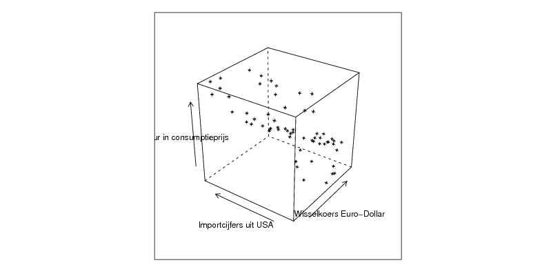
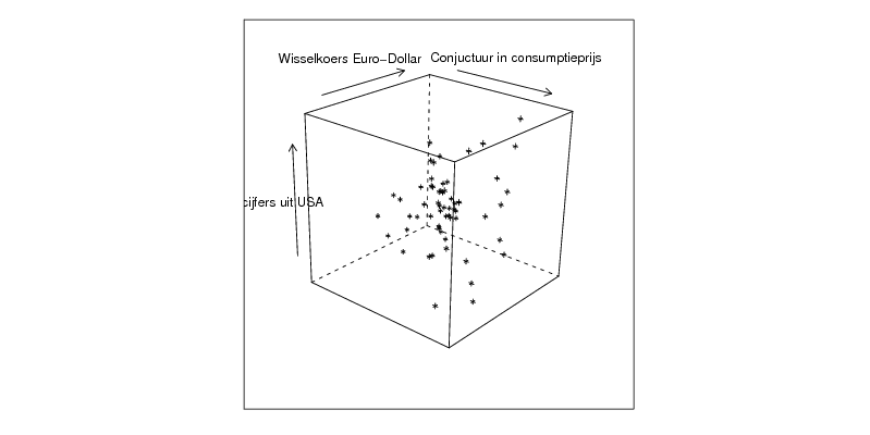
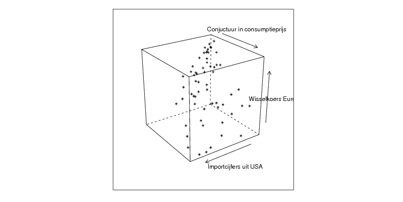
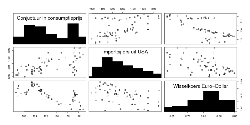
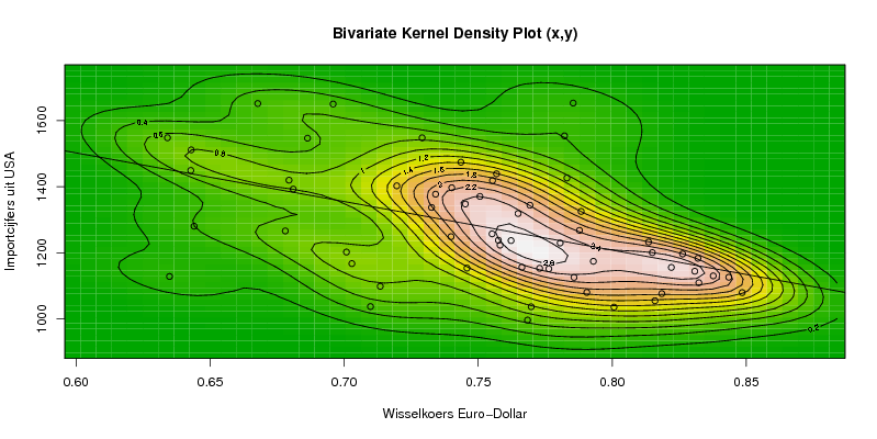
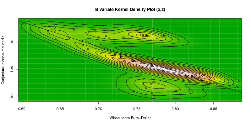
| Title produced by software | Trivariate Scatterplots | ||||||||||||||||||||
| Date of computation | Sun, 01 Nov 2009 12:01:36 -0700 | ||||||||||||||||||||
| Cite this page as follows | Statistical Computations at FreeStatistics.org, Office for Research Development and Education, URL https://freestatistics.org/blog/index.php?v=date/2009/Nov/01/t125710222470zranz9vv8nad0.htm/, Retrieved Mon, 06 May 2024 14:05:53 +0000 | ||||||||||||||||||||
| Statistical Computations at FreeStatistics.org, Office for Research Development and Education, URL https://freestatistics.org/blog/index.php?pk=52394, Retrieved Mon, 06 May 2024 14:05:53 +0000 | |||||||||||||||||||||
| QR Codes: | |||||||||||||||||||||
|
| |||||||||||||||||||||
| Original text written by user: | |||||||||||||||||||||
| IsPrivate? | No (this computation is public) | ||||||||||||||||||||
| User-defined keywords | |||||||||||||||||||||
| Estimated Impact | 187 | ||||||||||||||||||||
Tree of Dependent Computations | |||||||||||||||||||||
| Family? (F = Feedback message, R = changed R code, M = changed R Module, P = changed Parameters, D = changed Data) | |||||||||||||||||||||
| - [Bivariate Explorative Data Analysis] [WS 4 module 2] [2009-10-26 21:23:44] [830e13ac5e5ac1e5b21c6af0c149b21d] - RMPD [Partial Correlation] [WS 5 ] [2009-10-30 20:36:39] [023d83ebdf42a2acf423907b4076e8a1] - RMPD [Trivariate Scatterplots] [WS 5 triv] [2009-11-01 19:01:36] [51118f1042b56b16d340924f16263174] [Current] - RMP [Partial Correlation] [SHWWS5review4] [2009-11-06 10:24:33] [a66d3a79ef9e5308cd94a469bc5ca464] | |||||||||||||||||||||
| Feedback Forum | |||||||||||||||||||||
Post a new message | |||||||||||||||||||||
Dataset | |||||||||||||||||||||
| Dataseries X: | |||||||||||||||||||||
0.818465 0.800641 0.769764 0.745823 0.762253 0.768403 0.757518 0.772917 0.787774 0.82203 0.830772 0.813537 0.815927 0.832293 0.848464 0.843455 0.826241 0.837661 0.831947 0.81493 0.783085 0.790514 0.788395 0.780579 0.785731 0.792959 0.776337 0.75683 0.76929 0.764877 0.755173 0.739864 0.740138 0.745212 0.729076 0.734107 0.719632 0.702889 0.681013 0.686342 0.67944 0.678058 0.644039 0.63488 0.642797 0.642963 0.634115 0.66778 0.695894 0.750638 0.785423 0.74355 0.755344 0.782167 0.766284 0.75815 0.732601 0.71347 0.709824 0.700869 | |||||||||||||||||||||
| Dataseries Y: | |||||||||||||||||||||
1076.7 1035.9 1037 1154 1237.2 996.6 1238.2 1153.4 1268.1 1156 1144.5 1232.9 1055.2 1109.7 1079.8 1126.3 1196.8 1130.4 1183.6 1200.9 1426.6 1080.4 1325.4 1230 1125.9 1174.5 1151.9 1439.3 1344.3 1319.1 1257.6 1249.1 1397.1 1348 1548.2 1377.6 1402.9 1167.6 1392.9 1547 1420 1266.4 1280.8 1128.6 1449.5 1511.7 1548.3 1652 1650.5 1370.8 1653.3 1474.3 1418.8 1554.1 1156.6 1223.4 1337.5 1098.9 1037.6 1202.5 | |||||||||||||||||||||
| Dataseries Z: | |||||||||||||||||||||
101.01 100.88 100.55 100.82 101.5 102.16 102.39 102.54 102.85 103.47 103.57 103.69 103.5 103.47 103.45 103.48 103.93 103.89 104.4 104.79 104.77 105.13 105.26 104.96 104.75 105.01 105.15 105.2 105.77 105.78 106.26 106.13 106.12 106.57 106.44 106.54 107.1 108.1 108.4 108.84 109.62 110.42 110.67 111.66 112.28 112.87 112.18 112.36 112.16 111.49 111.25 111.36 111.74 111.1 111.33 111.25 111.04 110.97 111.31 111.02 | |||||||||||||||||||||
Tables (Output of Computation) | |||||||||||||||||||||
| |||||||||||||||||||||
Figures (Output of Computation) | |||||||||||||||||||||
Input Parameters & R Code | |||||||||||||||||||||
| Parameters (Session): | |||||||||||||||||||||
| par1 = 50 ; par2 = 50 ; par3 = Y ; par4 = Y ; par5 = Wisselkoers Euro-Dollar ; par6 = Importcijfers uit USA ; par7 = Conjuctuur in consumptieprijs ; | |||||||||||||||||||||
| Parameters (R input): | |||||||||||||||||||||
| par1 = 50 ; par2 = 50 ; par3 = Y ; par4 = Y ; par5 = Wisselkoers Euro-Dollar ; par6 = Importcijfers uit USA ; par7 = Conjuctuur in consumptieprijs ; | |||||||||||||||||||||
| R code (references can be found in the software module): | |||||||||||||||||||||
x <- array(x,dim=c(length(x),1)) | |||||||||||||||||||||