Free Statistics

of Irreproducible Research!

Author's title

Totale industri�le productie index met basis jaar = 2000 (periode 31/1 2004...

Author

*Unverified author*

R Software Module

rwasp_autocorrelation.wasp

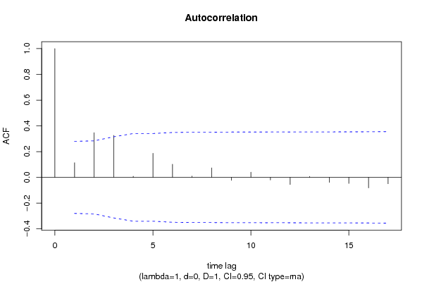
Title produced by software

(Partial) Autocorrelation Function

Date of computation

Thu, 26 Nov 2009 02:03:46 -0700

Cite this page as follows

Statistical Computations at FreeStatistics.org, Office for Research Development and Education, URL https://freestatistics.org/blog/index.php?v=date/2009/Nov/26/t12592263097y2xnf44ey0hdv5.htm/, Retrieved Mon, 29 Apr 2024 07:48:14 +0000

Statistical Computations at FreeStatistics.org, Office for Research Development and Education, URL https://freestatistics.org/blog/index.php?pk=59715, Retrieved Mon, 29 Apr 2024 07:48:14 +0000

QR Codes:

Paste this QR Code to cite your computation.

Original text written by user:

IsPrivate?

No (this computation is public)

User-defined keywords

Estimated Impact

168

Family? (F = Feedback message, R = changed R code, M = changed R Module, P = changed Parameters, D = changed Data)

-     [Univariate Explorative Data Analysis] [Run Sequence gebo...] [2008-12-12 13:32:37] [76963dc1903f0f612b6153510a3818cf]
- R  D  [Univariate Explorative Data Analysis] [Run Sequence gebo...] [2008-12-17 12:14:40] [76963dc1903f0f612b6153510a3818cf]
-         [Univariate Explorative Data Analysis] [Run Sequence Plot...] [2008-12-22 18:19:51] [1ce0d16c8f4225c977b42c8fa93bc163]
- RMP       [(Partial) Autocorrelation Function] [Identifying Integ...] [2009-11-22 12:19:56] [b98453cac15ba1066b407e146608df68]
- R PD          [(Partial) Autocorrelation Function] [Totale industri�l...] [2009-11-26 09:03:46] [d41d8cd98f00b204e9800998ecf8427e] [Current]
- R P             [(Partial) Autocorrelation Function] [Method 1:ACF - d=...] [2009-11-27 13:43:54] [74be16979710d4c4e7c6647856088456] 
- R                 [(Partial) Autocorrelation Function] [Method 1:ACF - d=...] [2009-12-20 19:46:18] [77c4589624c8ef9dff4002b842437335] 
- R P             [(Partial) Autocorrelation Function] [Method-1: ACF - d...] [2009-11-27 13:46:33] [74be16979710d4c4e7c6647856088456] 
- R P               [(Partial) Autocorrelation Function] [Method-1: ACF - d...] [2009-12-20 19:48:42] [77c4589624c8ef9dff4002b842437335] 
- R P             [(Partial) Autocorrelation Function] [Method-1: ACF - d...] [2009-11-27 13:48:51] [74be16979710d4c4e7c6647856088456] 
- R P               [(Partial) Autocorrelation Function] [Method-1: ACF - d...] [2009-12-20 19:50:14] [77c4589624c8ef9dff4002b842437335] 

Feedback Forum

Post a new message

Dataseries X:

Download CSV

Histogram

Boxplots

Summary of computational transaction
Raw Input	view raw input (R code)
Raw Output	view raw output of R engine
Computing time	2 seconds
R Server	'Gwilym Jenkins' @ 72.249.127.135

\begin{tabular}{lllllllll}
\hline
Summary of computational transaction \tabularnewline
Raw Input & view raw input (R code)  \tabularnewline
Raw Output & view raw output of R engine  \tabularnewline
Computing time & 2 seconds \tabularnewline
R Server & 'Gwilym Jenkins' @ 72.249.127.135 \tabularnewline
\hline
\end{tabular}
%Source: https://freestatistics.org/blog/index.php?pk=59715&T=0

[TABLE]
[ROW][C]Summary of computational transaction[/C][/ROW]
[ROW][C]Raw Input[/C][C]view raw input (R code) [/C][/ROW]
[ROW][C]Raw Output[/C][C]view raw output of R engine [/C][/ROW]
[ROW][C]Computing time[/C][C]2 seconds[/C][/ROW]
[ROW][C]R Server[/C][C]'Gwilym Jenkins' @ 72.249.127.135[/C][/ROW]
[/TABLE]
Source: https://freestatistics.org/blog/index.php?pk=59715&T=0

Globally Unique Identifier (entire table): ba.freestatistics.org/blog/index.php?pk=59715&T=0

As an alternative you can also use a QR Code:

The GUIDs for individual cells are displayed in the table below:

Summary of computational transaction
Raw Input	view raw input (R code)
Raw Output	view raw output of R engine
Computing time	2 seconds
R Server	'Gwilym Jenkins' @ 72.249.127.135

Autocorrelation Function
Time lag k	ACF(k)	T-STAT	P-value
1	0.114099	0.7987	0.214161
2	0.347255	2.4308	0.009386
3	0.325683	2.2798	0.013506
4	0.008725	0.0611	0.475775
5	0.187089	1.3096	0.098215
6	0.101996	0.714	0.239317
7	0.009668	0.0677	0.473159
8	0.073744	0.5162	0.304014
9	-0.023383	-0.1637	0.435329
10	0.040363	0.2825	0.389358
11	-0.020399	-0.1428	0.44352
12	-0.054968	-0.3848	0.351035
13	0.007439	0.0521	0.479341
14	-0.038736	-0.2712	0.393707
15	-0.046939	-0.3286	0.371939
16	-0.082102	-0.5747	0.284057
17	-0.050101	-0.3507	0.363656

\begin{tabular}{lllllllll}
\hline
Autocorrelation Function \tabularnewline
Time lag k & ACF(k) & T-STAT & P-value \tabularnewline
1 & 0.114099 & 0.7987 & 0.214161 \tabularnewline
2 & 0.347255 & 2.4308 & 0.009386 \tabularnewline
3 & 0.325683 & 2.2798 & 0.013506 \tabularnewline
4 & 0.008725 & 0.0611 & 0.475775 \tabularnewline
5 & 0.187089 & 1.3096 & 0.098215 \tabularnewline
6 & 0.101996 & 0.714 & 0.239317 \tabularnewline
7 & 0.009668 & 0.0677 & 0.473159 \tabularnewline
8 & 0.073744 & 0.5162 & 0.304014 \tabularnewline
9 & -0.023383 & -0.1637 & 0.435329 \tabularnewline
10 & 0.040363 & 0.2825 & 0.389358 \tabularnewline
11 & -0.020399 & -0.1428 & 0.44352 \tabularnewline
12 & -0.054968 & -0.3848 & 0.351035 \tabularnewline
13 & 0.007439 & 0.0521 & 0.479341 \tabularnewline
14 & -0.038736 & -0.2712 & 0.393707 \tabularnewline
15 & -0.046939 & -0.3286 & 0.371939 \tabularnewline
16 & -0.082102 & -0.5747 & 0.284057 \tabularnewline
17 & -0.050101 & -0.3507 & 0.363656 \tabularnewline
\hline
\end{tabular}
%Source: https://freestatistics.org/blog/index.php?pk=59715&T=1

[TABLE]
[ROW][C]Autocorrelation Function[/C][/ROW]
[ROW][C]Time lag k[/C][C]ACF(k)[/C][C]T-STAT[/C][C]P-value[/C][/ROW]
[ROW][C]1[/C][C]0.114099[/C][C]0.7987[/C][C]0.214161[/C][/ROW]
[ROW][C]2[/C][C]0.347255[/C][C]2.4308[/C][C]0.009386[/C][/ROW]
[ROW][C]3[/C][C]0.325683[/C][C]2.2798[/C][C]0.013506[/C][/ROW]
[ROW][C]4[/C][C]0.008725[/C][C]0.0611[/C][C]0.475775[/C][/ROW]
[ROW][C]5[/C][C]0.187089[/C][C]1.3096[/C][C]0.098215[/C][/ROW]
[ROW][C]6[/C][C]0.101996[/C][C]0.714[/C][C]0.239317[/C][/ROW]
[ROW][C]7[/C][C]0.009668[/C][C]0.0677[/C][C]0.473159[/C][/ROW]
[ROW][C]8[/C][C]0.073744[/C][C]0.5162[/C][C]0.304014[/C][/ROW]
[ROW][C]9[/C][C]-0.023383[/C][C]-0.1637[/C][C]0.435329[/C][/ROW]
[ROW][C]10[/C][C]0.040363[/C][C]0.2825[/C][C]0.389358[/C][/ROW]
[ROW][C]11[/C][C]-0.020399[/C][C]-0.1428[/C][C]0.44352[/C][/ROW]
[ROW][C]12[/C][C]-0.054968[/C][C]-0.3848[/C][C]0.351035[/C][/ROW]
[ROW][C]13[/C][C]0.007439[/C][C]0.0521[/C][C]0.479341[/C][/ROW]
[ROW][C]14[/C][C]-0.038736[/C][C]-0.2712[/C][C]0.393707[/C][/ROW]
[ROW][C]15[/C][C]-0.046939[/C][C]-0.3286[/C][C]0.371939[/C][/ROW]
[ROW][C]16[/C][C]-0.082102[/C][C]-0.5747[/C][C]0.284057[/C][/ROW]
[ROW][C]17[/C][C]-0.050101[/C][C]-0.3507[/C][C]0.363656[/C][/ROW]
[/TABLE]
Source: https://freestatistics.org/blog/index.php?pk=59715&T=1

Globally Unique Identifier (entire table): ba.freestatistics.org/blog/index.php?pk=59715&T=1

As an alternative you can also use a QR Code:

The GUIDs for individual cells are displayed in the table below:

Autocorrelation Function
Time lag k	ACF(k)	T-STAT	P-value
1	0.114099	0.7987	0.214161
2	0.347255	2.4308	0.009386
3	0.325683	2.2798	0.013506
4	0.008725	0.0611	0.475775
5	0.187089	1.3096	0.098215
6	0.101996	0.714	0.239317
7	0.009668	0.0677	0.473159
8	0.073744	0.5162	0.304014
9	-0.023383	-0.1637	0.435329
10	0.040363	0.2825	0.389358
11	-0.020399	-0.1428	0.44352
12	-0.054968	-0.3848	0.351035
13	0.007439	0.0521	0.479341
14	-0.038736	-0.2712	0.393707
15	-0.046939	-0.3286	0.371939
16	-0.082102	-0.5747	0.284057
17	-0.050101	-0.3507	0.363656

Partial Autocorrelation Function
Time lag k	PACF(k)	T-STAT	P-value
1	0.114099	0.7987	0.214161
2	0.338645	2.3705	0.010871
3	0.298514	2.0896	0.020934
4	-0.159263	-1.1148	0.135178
5	-0.021302	-0.1491	0.441039
6	0.070182	0.4913	0.312712
7	-0.008512	-0.0596	0.476364
8	-0.043346	-0.3034	0.381428
9	-0.054632	-0.3824	0.3519
10	0.062426	0.437	0.332023
11	-0.022061	-0.1544	0.438953
12	-0.081553	-0.5709	0.285349
13	0.002075	0.0145	0.494234
14	0.044189	0.3093	0.379194
15	-0.030115	-0.2108	0.416956
16	-0.1283	-0.8981	0.186763
17	0.002743	0.0192	0.492379

\begin{tabular}{lllllllll}
\hline
Partial Autocorrelation Function \tabularnewline
Time lag k & PACF(k) & T-STAT & P-value \tabularnewline
1 & 0.114099 & 0.7987 & 0.214161 \tabularnewline
2 & 0.338645 & 2.3705 & 0.010871 \tabularnewline
3 & 0.298514 & 2.0896 & 0.020934 \tabularnewline
4 & -0.159263 & -1.1148 & 0.135178 \tabularnewline
5 & -0.021302 & -0.1491 & 0.441039 \tabularnewline
6 & 0.070182 & 0.4913 & 0.312712 \tabularnewline
7 & -0.008512 & -0.0596 & 0.476364 \tabularnewline
8 & -0.043346 & -0.3034 & 0.381428 \tabularnewline
9 & -0.054632 & -0.3824 & 0.3519 \tabularnewline
10 & 0.062426 & 0.437 & 0.332023 \tabularnewline
11 & -0.022061 & -0.1544 & 0.438953 \tabularnewline
12 & -0.081553 & -0.5709 & 0.285349 \tabularnewline
13 & 0.002075 & 0.0145 & 0.494234 \tabularnewline
14 & 0.044189 & 0.3093 & 0.379194 \tabularnewline
15 & -0.030115 & -0.2108 & 0.416956 \tabularnewline
16 & -0.1283 & -0.8981 & 0.186763 \tabularnewline
17 & 0.002743 & 0.0192 & 0.492379 \tabularnewline
\hline
\end{tabular}
%Source: https://freestatistics.org/blog/index.php?pk=59715&T=2

[TABLE]
[ROW][C]Partial Autocorrelation Function[/C][/ROW]
[ROW][C]Time lag k[/C][C]PACF(k)[/C][C]T-STAT[/C][C]P-value[/C][/ROW]
[ROW][C]1[/C][C]0.114099[/C][C]0.7987[/C][C]0.214161[/C][/ROW]
[ROW][C]2[/C][C]0.338645[/C][C]2.3705[/C][C]0.010871[/C][/ROW]
[ROW][C]3[/C][C]0.298514[/C][C]2.0896[/C][C]0.020934[/C][/ROW]
[ROW][C]4[/C][C]-0.159263[/C][C]-1.1148[/C][C]0.135178[/C][/ROW]
[ROW][C]5[/C][C]-0.021302[/C][C]-0.1491[/C][C]0.441039[/C][/ROW]
[ROW][C]6[/C][C]0.070182[/C][C]0.4913[/C][C]0.312712[/C][/ROW]
[ROW][C]7[/C][C]-0.008512[/C][C]-0.0596[/C][C]0.476364[/C][/ROW]
[ROW][C]8[/C][C]-0.043346[/C][C]-0.3034[/C][C]0.381428[/C][/ROW]
[ROW][C]9[/C][C]-0.054632[/C][C]-0.3824[/C][C]0.3519[/C][/ROW]
[ROW][C]10[/C][C]0.062426[/C][C]0.437[/C][C]0.332023[/C][/ROW]
[ROW][C]11[/C][C]-0.022061[/C][C]-0.1544[/C][C]0.438953[/C][/ROW]
[ROW][C]12[/C][C]-0.081553[/C][C]-0.5709[/C][C]0.285349[/C][/ROW]
[ROW][C]13[/C][C]0.002075[/C][C]0.0145[/C][C]0.494234[/C][/ROW]
[ROW][C]14[/C][C]0.044189[/C][C]0.3093[/C][C]0.379194[/C][/ROW]
[ROW][C]15[/C][C]-0.030115[/C][C]-0.2108[/C][C]0.416956[/C][/ROW]
[ROW][C]16[/C][C]-0.1283[/C][C]-0.8981[/C][C]0.186763[/C][/ROW]
[ROW][C]17[/C][C]0.002743[/C][C]0.0192[/C][C]0.492379[/C][/ROW]
[/TABLE]
Source: https://freestatistics.org/blog/index.php?pk=59715&T=2

Globally Unique Identifier (entire table): ba.freestatistics.org/blog/index.php?pk=59715&T=2

As an alternative you can also use a QR Code:

The GUIDs for individual cells are displayed in the table below:

Partial Autocorrelation Function
Time lag k	PACF(k)	T-STAT	P-value
1	0.114099	0.7987	0.214161
2	0.338645	2.3705	0.010871
3	0.298514	2.0896	0.020934
4	-0.159263	-1.1148	0.135178
5	-0.021302	-0.1491	0.441039
6	0.070182	0.4913	0.312712
7	-0.008512	-0.0596	0.476364
8	-0.043346	-0.3034	0.381428
9	-0.054632	-0.3824	0.3519
10	0.062426	0.437	0.332023
11	-0.022061	-0.1544	0.438953
12	-0.081553	-0.5709	0.285349
13	0.002075	0.0145	0.494234
14	0.044189	0.3093	0.379194
15	-0.030115	-0.2108	0.416956
16	-0.1283	-0.8981	0.186763
17	0.002743	0.0192	0.492379

Figure 1

PNG link

Postscript link

PDF link

Figure 2

PNG link

Postscript link

PDF link

Parameters (Session):

par1 = Default ; par2 = 1 ; par3 = 0 ; par4 = 1 ; par5 = 12 ; par6 = MA ; par7 = 0.95 ;

Parameters (R input):

par1 = Default ; par2 = 1 ; par3 = 0 ; par4 = 1 ; par5 = 12 ; par6 = MA ; par7 = 0.95 ;

R code (references can be found in the software module):

if (par1 == 'Default') {
par1 = 10*log10(length(x))
} else {
par1 <- as.numeric(par1)
}
par2 <- as.numeric(par2)
par3 <- as.numeric(par3)
par4 <- as.numeric(par4)
par5 <- as.numeric(par5)
if (par6 == 'White Noise') par6 <- 'white' else par6 <- 'ma'
par7 <- as.numeric(par7)
if (par2 == 0) {
x <- log(x)
} else {
x <- (x ^ par2 - 1) / par2
}
if (par3 > 0) x <- diff(x,lag=1,difference=par3)
if (par4 > 0) x <- diff(x,lag=par5,difference=par4)
bitmap(file='pic1.png')
racf <- acf(x, par1, main='Autocorrelation', xlab='time lag', ylab='ACF', ci.type=par6, ci=par7, sub=paste('(lambda=',par2,', d=',par3,', D=',par4,', CI=', par7, ', CI type=',par6,')',sep=''))
dev.off()
bitmap(file='pic2.png')
rpacf <- pacf(x,par1,main='Partial Autocorrelation',xlab='lags',ylab='PACF')
dev.off()
(myacf <- c(racf$acf))
(mypacf <- c(rpacf$acf))
lengthx <- length(x)
sqrtn <- sqrt(lengthx)
load(file='createtable')
a<-table.start()
a<-table.row.start(a)
a<-table.element(a,'Autocorrelation Function',4,TRUE)
a<-table.row.end(a)
a<-table.row.start(a)
a<-table.element(a,'Time lag k',header=TRUE)
a<-table.element(a,hyperlink('basics.htm','ACF(k)','click here for more information about the Autocorrelation Function'),header=TRUE)
a<-table.element(a,'T-STAT',header=TRUE)
a<-table.element(a,'P-value',header=TRUE)
a<-table.row.end(a)
for (i in 2:(par1+1)) {
a<-table.row.start(a)
a<-table.element(a,i-1,header=TRUE)
a<-table.element(a,round(myacf[i],6))
mytstat <- myacf[i]*sqrtn
a<-table.element(a,round(mytstat,4))
a<-table.element(a,round(1-pt(abs(mytstat),lengthx),6))
a<-table.row.end(a)
}
a<-table.end(a)
table.save(a,file='mytable.tab')
a<-table.start()
a<-table.row.start(a)
a<-table.element(a,'Partial Autocorrelation Function',4,TRUE)
a<-table.row.end(a)
a<-table.row.start(a)
a<-table.element(a,'Time lag k',header=TRUE)
a<-table.element(a,hyperlink('basics.htm','PACF(k)','click here for more information about the Partial Autocorrelation Function'),header=TRUE)
a<-table.element(a,'T-STAT',header=TRUE)
a<-table.element(a,'P-value',header=TRUE)
a<-table.row.end(a)
for (i in 1:par1) {
a<-table.row.start(a)
a<-table.element(a,i,header=TRUE)
a<-table.element(a,round(mypacf[i],6))
mytstat <- mypacf[i]*sqrtn
a<-table.element(a,round(mytstat,4))
a<-table.element(a,round(1-pt(abs(mytstat),lengthx),6))
a<-table.row.end(a)
}
a<-table.end(a)
table.save(a,file='mytable1.tab')

Free Statistics

Description of Statistical Computation

Totale industri�le productie index met basis jaar = 2000 (periode 31/1 2004...

Tree of Dependent Computations

Dataset

Tables (Output of Computation)

Figures (Output of Computation)

Input Parameters & R Code