Repository of Reproducible Computations

Free Statistics

of Irreproducible Research!

Author's title

Author

*The author of this computation has been verified*

R Software Module

rwasp_autocorrelation.wasp

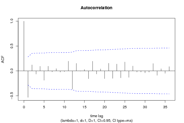
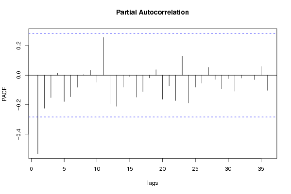
Title produced by software

(Partial) Autocorrelation Function

Date of computation

Thu, 26 Nov 2009 03:10:06 -0700

Cite this page as follows

Statistical Computations at FreeStatistics.org, Office for Research Development and Education, URL https://freestatistics.org/blog/index.php?v=date/2009/Nov/26/t1259230249ij5hzxsdj84otcs.htm/, Retrieved Sun, 28 Apr 2024 22:14:38 +0000

Statistical Computations at FreeStatistics.org, Office for Research Development and Education, URL https://freestatistics.org/blog/index.php?pk=59767, Retrieved Sun, 28 Apr 2024 22:14:38 +0000

QR Codes:

Paste this QR Code to cite your computation.

Original text written by user:

IsPrivate?

No (this computation is public)

User-defined keywords

Estimated Impact

143

Family? (F = Feedback message, R = changed R code, M = changed R Module, P = changed Parameters, D = changed Data)

-     [Univariate Explorative Data Analysis] [Run Sequence gebo...] [2008-12-12 13:32:37] [76963dc1903f0f612b6153510a3818cf]
- R  D  [Univariate Explorative Data Analysis] [Run Sequence gebo...] [2008-12-17 12:14:40] [76963dc1903f0f612b6153510a3818cf]
-         [Univariate Explorative Data Analysis] [Run Sequence Plot...] [2008-12-22 18:19:51] [1ce0d16c8f4225c977b42c8fa93bc163]
- RMP       [(Partial) Autocorrelation Function] [Identifying Integ...] [2009-11-22 12:26:39] [b98453cac15ba1066b407e146608df68]
-    D          [(Partial) Autocorrelation Function] [ACF met: d=1, D=1...] [2009-11-26 10:10:06] [371dc2189c569d90e2c1567f632c3ec0] [Current]
-   P             [(Partial) Autocorrelation Function] [ACF met: d=1, D=1...] [2009-12-19 11:16:17] [34d27ebe78dc2d31581e8710befe8733] 

Feedback Forum

Post a new message

Dataseries X:

Download CSV

Histogram

Boxplots

Summary of computational transaction
Raw Input	view raw input (R code)
Raw Output	view raw output of R engine
Computing time	1 seconds
R Server	'Gwilym Jenkins' @ 72.249.127.135

\begin{tabular}{lllllllll}
\hline
Summary of computational transaction \tabularnewline
Raw Input & view raw input (R code)  \tabularnewline
Raw Output & view raw output of R engine  \tabularnewline
Computing time & 1 seconds \tabularnewline
R Server & 'Gwilym Jenkins' @ 72.249.127.135 \tabularnewline
\hline
\end{tabular}
%Source: https://freestatistics.org/blog/index.php?pk=59767&T=0

[TABLE]
[ROW][C]Summary of computational transaction[/C][/ROW]
[ROW][C]Raw Input[/C][C]view raw input (R code) [/C][/ROW]
[ROW][C]Raw Output[/C][C]view raw output of R engine [/C][/ROW]
[ROW][C]Computing time[/C][C]1 seconds[/C][/ROW]
[ROW][C]R Server[/C][C]'Gwilym Jenkins' @ 72.249.127.135[/C][/ROW]
[/TABLE]
Source: https://freestatistics.org/blog/index.php?pk=59767&T=0

Globally Unique Identifier (entire table): ba.freestatistics.org/blog/index.php?pk=59767&T=0

As an alternative you can also use a QR Code:

The GUIDs for individual cells are displayed in the table below:

Summary of computational transaction
Raw Input	view raw input (R code)
Raw Output	view raw output of R engine
Computing time	1 seconds
R Server	'Gwilym Jenkins' @ 72.249.127.135

Autocorrelation Function
Time lag k	ACF(k)	T-STAT	P-value
1	-0.531404	-3.6817	0.000293
2	0.121571	0.8423	0.201907
3	-0.06376	-0.4417	0.33033
4	0.094536	0.655	0.257809
5	-0.187874	-1.3016	0.099628
6	0.095275	0.6601	0.256177
7	-0.018754	-0.1299	0.448581
8	0.046874	0.3248	0.37339
9	-0.023328	-0.1616	0.436142
10	-0.014478	-0.1003	0.460261
11	0.196162	1.3591	0.090241
12	-0.367193	-2.544	0.007117
13	0.152388	1.0558	0.148177
14	-0.002995	-0.0208	0.491765
15	0.029399	0.2037	0.419731
16	-0.15667	-1.0854	0.141574
17	0.195231	1.3526	0.09126
18	-0.062142	-0.4305	0.334367
19	0.041577	0.2881	0.387273
20	-0.155282	-1.0758	0.143692
21	0.155047	1.0742	0.144053
22	-0.14971	-1.0372	0.152415
23	0.139159	0.9641	0.169909
24	-0.139277	-0.9649	0.169706
25	0.180006	1.2471	0.109203
26	-0.129564	-0.8976	0.186927
27	0.098977	0.6857	0.248091
28	-0.021283	-0.1475	0.441696
29	-0.021456	-0.1487	0.441226
30	-0.039309	-0.2723	0.393264
31	-0.023557	-0.1632	0.435521
32	0.149306	1.0344	0.153062
33	-0.087823	-0.6085	0.272878
34	0.044944	0.3114	0.378429
35	-0.047835	-0.3314	0.370888
36	0.087734	0.6078	0.273079

\begin{tabular}{lllllllll}
\hline
Autocorrelation Function \tabularnewline
Time lag k & ACF(k) & T-STAT & P-value \tabularnewline
1 & -0.531404 & -3.6817 & 0.000293 \tabularnewline
2 & 0.121571 & 0.8423 & 0.201907 \tabularnewline
3 & -0.06376 & -0.4417 & 0.33033 \tabularnewline
4 & 0.094536 & 0.655 & 0.257809 \tabularnewline
5 & -0.187874 & -1.3016 & 0.099628 \tabularnewline
6 & 0.095275 & 0.6601 & 0.256177 \tabularnewline
7 & -0.018754 & -0.1299 & 0.448581 \tabularnewline
8 & 0.046874 & 0.3248 & 0.37339 \tabularnewline
9 & -0.023328 & -0.1616 & 0.436142 \tabularnewline
10 & -0.014478 & -0.1003 & 0.460261 \tabularnewline
11 & 0.196162 & 1.3591 & 0.090241 \tabularnewline
12 & -0.367193 & -2.544 & 0.007117 \tabularnewline
13 & 0.152388 & 1.0558 & 0.148177 \tabularnewline
14 & -0.002995 & -0.0208 & 0.491765 \tabularnewline
15 & 0.029399 & 0.2037 & 0.419731 \tabularnewline
16 & -0.15667 & -1.0854 & 0.141574 \tabularnewline
17 & 0.195231 & 1.3526 & 0.09126 \tabularnewline
18 & -0.062142 & -0.4305 & 0.334367 \tabularnewline
19 & 0.041577 & 0.2881 & 0.387273 \tabularnewline
20 & -0.155282 & -1.0758 & 0.143692 \tabularnewline
21 & 0.155047 & 1.0742 & 0.144053 \tabularnewline
22 & -0.14971 & -1.0372 & 0.152415 \tabularnewline
23 & 0.139159 & 0.9641 & 0.169909 \tabularnewline
24 & -0.139277 & -0.9649 & 0.169706 \tabularnewline
25 & 0.180006 & 1.2471 & 0.109203 \tabularnewline
26 & -0.129564 & -0.8976 & 0.186927 \tabularnewline
27 & 0.098977 & 0.6857 & 0.248091 \tabularnewline
28 & -0.021283 & -0.1475 & 0.441696 \tabularnewline
29 & -0.021456 & -0.1487 & 0.441226 \tabularnewline
30 & -0.039309 & -0.2723 & 0.393264 \tabularnewline
31 & -0.023557 & -0.1632 & 0.435521 \tabularnewline
32 & 0.149306 & 1.0344 & 0.153062 \tabularnewline
33 & -0.087823 & -0.6085 & 0.272878 \tabularnewline
34 & 0.044944 & 0.3114 & 0.378429 \tabularnewline
35 & -0.047835 & -0.3314 & 0.370888 \tabularnewline
36 & 0.087734 & 0.6078 & 0.273079 \tabularnewline
\hline
\end{tabular}
%Source: https://freestatistics.org/blog/index.php?pk=59767&T=1

[TABLE]
[ROW][C]Autocorrelation Function[/C][/ROW]
[ROW][C]Time lag k[/C][C]ACF(k)[/C][C]T-STAT[/C][C]P-value[/C][/ROW]
[ROW][C]1[/C][C]-0.531404[/C][C]-3.6817[/C][C]0.000293[/C][/ROW]
[ROW][C]2[/C][C]0.121571[/C][C]0.8423[/C][C]0.201907[/C][/ROW]
[ROW][C]3[/C][C]-0.06376[/C][C]-0.4417[/C][C]0.33033[/C][/ROW]
[ROW][C]4[/C][C]0.094536[/C][C]0.655[/C][C]0.257809[/C][/ROW]
[ROW][C]5[/C][C]-0.187874[/C][C]-1.3016[/C][C]0.099628[/C][/ROW]
[ROW][C]6[/C][C]0.095275[/C][C]0.6601[/C][C]0.256177[/C][/ROW]
[ROW][C]7[/C][C]-0.018754[/C][C]-0.1299[/C][C]0.448581[/C][/ROW]
[ROW][C]8[/C][C]0.046874[/C][C]0.3248[/C][C]0.37339[/C][/ROW]
[ROW][C]9[/C][C]-0.023328[/C][C]-0.1616[/C][C]0.436142[/C][/ROW]
[ROW][C]10[/C][C]-0.014478[/C][C]-0.1003[/C][C]0.460261[/C][/ROW]
[ROW][C]11[/C][C]0.196162[/C][C]1.3591[/C][C]0.090241[/C][/ROW]
[ROW][C]12[/C][C]-0.367193[/C][C]-2.544[/C][C]0.007117[/C][/ROW]
[ROW][C]13[/C][C]0.152388[/C][C]1.0558[/C][C]0.148177[/C][/ROW]
[ROW][C]14[/C][C]-0.002995[/C][C]-0.0208[/C][C]0.491765[/C][/ROW]
[ROW][C]15[/C][C]0.029399[/C][C]0.2037[/C][C]0.419731[/C][/ROW]
[ROW][C]16[/C][C]-0.15667[/C][C]-1.0854[/C][C]0.141574[/C][/ROW]
[ROW][C]17[/C][C]0.195231[/C][C]1.3526[/C][C]0.09126[/C][/ROW]
[ROW][C]18[/C][C]-0.062142[/C][C]-0.4305[/C][C]0.334367[/C][/ROW]
[ROW][C]19[/C][C]0.041577[/C][C]0.2881[/C][C]0.387273[/C][/ROW]
[ROW][C]20[/C][C]-0.155282[/C][C]-1.0758[/C][C]0.143692[/C][/ROW]
[ROW][C]21[/C][C]0.155047[/C][C]1.0742[/C][C]0.144053[/C][/ROW]
[ROW][C]22[/C][C]-0.14971[/C][C]-1.0372[/C][C]0.152415[/C][/ROW]
[ROW][C]23[/C][C]0.139159[/C][C]0.9641[/C][C]0.169909[/C][/ROW]
[ROW][C]24[/C][C]-0.139277[/C][C]-0.9649[/C][C]0.169706[/C][/ROW]
[ROW][C]25[/C][C]0.180006[/C][C]1.2471[/C][C]0.109203[/C][/ROW]
[ROW][C]26[/C][C]-0.129564[/C][C]-0.8976[/C][C]0.186927[/C][/ROW]
[ROW][C]27[/C][C]0.098977[/C][C]0.6857[/C][C]0.248091[/C][/ROW]
[ROW][C]28[/C][C]-0.021283[/C][C]-0.1475[/C][C]0.441696[/C][/ROW]
[ROW][C]29[/C][C]-0.021456[/C][C]-0.1487[/C][C]0.441226[/C][/ROW]
[ROW][C]30[/C][C]-0.039309[/C][C]-0.2723[/C][C]0.393264[/C][/ROW]
[ROW][C]31[/C][C]-0.023557[/C][C]-0.1632[/C][C]0.435521[/C][/ROW]
[ROW][C]32[/C][C]0.149306[/C][C]1.0344[/C][C]0.153062[/C][/ROW]
[ROW][C]33[/C][C]-0.087823[/C][C]-0.6085[/C][C]0.272878[/C][/ROW]
[ROW][C]34[/C][C]0.044944[/C][C]0.3114[/C][C]0.378429[/C][/ROW]
[ROW][C]35[/C][C]-0.047835[/C][C]-0.3314[/C][C]0.370888[/C][/ROW]
[ROW][C]36[/C][C]0.087734[/C][C]0.6078[/C][C]0.273079[/C][/ROW]
[/TABLE]
Source: https://freestatistics.org/blog/index.php?pk=59767&T=1

Globally Unique Identifier (entire table): ba.freestatistics.org/blog/index.php?pk=59767&T=1

As an alternative you can also use a QR Code:

The GUIDs for individual cells are displayed in the table below:

Autocorrelation Function
Time lag k	ACF(k)	T-STAT	P-value
1	-0.531404	-3.6817	0.000293
2	0.121571	0.8423	0.201907
3	-0.06376	-0.4417	0.33033
4	0.094536	0.655	0.257809
5	-0.187874	-1.3016	0.099628
6	0.095275	0.6601	0.256177
7	-0.018754	-0.1299	0.448581
8	0.046874	0.3248	0.37339
9	-0.023328	-0.1616	0.436142
10	-0.014478	-0.1003	0.460261
11	0.196162	1.3591	0.090241
12	-0.367193	-2.544	0.007117
13	0.152388	1.0558	0.148177
14	-0.002995	-0.0208	0.491765
15	0.029399	0.2037	0.419731
16	-0.15667	-1.0854	0.141574
17	0.195231	1.3526	0.09126
18	-0.062142	-0.4305	0.334367
19	0.041577	0.2881	0.387273
20	-0.155282	-1.0758	0.143692
21	0.155047	1.0742	0.144053
22	-0.14971	-1.0372	0.152415
23	0.139159	0.9641	0.169909
24	-0.139277	-0.9649	0.169706
25	0.180006	1.2471	0.109203
26	-0.129564	-0.8976	0.186927
27	0.098977	0.6857	0.248091
28	-0.021283	-0.1475	0.441696
29	-0.021456	-0.1487	0.441226
30	-0.039309	-0.2723	0.393264
31	-0.023557	-0.1632	0.435521
32	0.149306	1.0344	0.153062
33	-0.087823	-0.6085	0.272878
34	0.044944	0.3114	0.378429
35	-0.047835	-0.3314	0.370888
36	0.087734	0.6078	0.273079

Partial Autocorrelation Function
Time lag k	PACF(k)	T-STAT	P-value
1	-0.531404	-3.6817	0.000293
2	-0.224104	-1.5526	0.06354
3	-0.152249	-1.0548	0.148396
4	0.013914	0.0964	0.461802
5	-0.178663	-1.2378	0.110903
6	-0.146628	-1.0159	0.157392
7	-0.0819	-0.5674	0.286536
8	0.00461	0.0319	0.487328
9	0.033538	0.2324	0.408623
10	-0.047927	-0.332	0.370651
11	0.255297	1.7687	0.041645
12	-0.194574	-1.348	0.091985
13	-0.211097	-1.4625	0.075058
14	-0.081524	-0.5648	0.287416
15	-0.011138	-0.0772	0.469407
16	-0.148739	-1.0305	0.153971
17	-0.111158	-0.7701	0.2225
18	-0.019046	-0.132	0.447787
19	0.037142	0.2573	0.399014
20	-0.163328	-1.1316	0.131718
21	-0.071635	-0.4963	0.310974
22	-0.172085	-1.1922	0.119514
23	0.129528	0.8974	0.186993
24	-0.188628	-1.3069	0.098744
25	-0.081524	-0.5648	0.287414
26	-0.05371	-0.3721	0.355723
27	0.053066	0.3676	0.357376
28	-0.028848	-0.1999	0.421214
29	-0.094133	-0.6522	0.2587
30	-0.023634	-0.1637	0.435311
31	-0.108756	-0.7535	0.22742
32	-0.019737	-0.1367	0.445903
33	0.06851	0.4746	0.318595
34	-0.030412	-0.2107	0.417008
35	0.059021	0.4089	0.342213
36	-0.103034	-0.7138	0.239392

\begin{tabular}{lllllllll}
\hline
Partial Autocorrelation Function \tabularnewline
Time lag k & PACF(k) & T-STAT & P-value \tabularnewline
1 & -0.531404 & -3.6817 & 0.000293 \tabularnewline
2 & -0.224104 & -1.5526 & 0.06354 \tabularnewline
3 & -0.152249 & -1.0548 & 0.148396 \tabularnewline
4 & 0.013914 & 0.0964 & 0.461802 \tabularnewline
5 & -0.178663 & -1.2378 & 0.110903 \tabularnewline
6 & -0.146628 & -1.0159 & 0.157392 \tabularnewline
7 & -0.0819 & -0.5674 & 0.286536 \tabularnewline
8 & 0.00461 & 0.0319 & 0.487328 \tabularnewline
9 & 0.033538 & 0.2324 & 0.408623 \tabularnewline
10 & -0.047927 & -0.332 & 0.370651 \tabularnewline
11 & 0.255297 & 1.7687 & 0.041645 \tabularnewline
12 & -0.194574 & -1.348 & 0.091985 \tabularnewline
13 & -0.211097 & -1.4625 & 0.075058 \tabularnewline
14 & -0.081524 & -0.5648 & 0.287416 \tabularnewline
15 & -0.011138 & -0.0772 & 0.469407 \tabularnewline
16 & -0.148739 & -1.0305 & 0.153971 \tabularnewline
17 & -0.111158 & -0.7701 & 0.2225 \tabularnewline
18 & -0.019046 & -0.132 & 0.447787 \tabularnewline
19 & 0.037142 & 0.2573 & 0.399014 \tabularnewline
20 & -0.163328 & -1.1316 & 0.131718 \tabularnewline
21 & -0.071635 & -0.4963 & 0.310974 \tabularnewline
22 & -0.172085 & -1.1922 & 0.119514 \tabularnewline
23 & 0.129528 & 0.8974 & 0.186993 \tabularnewline
24 & -0.188628 & -1.3069 & 0.098744 \tabularnewline
25 & -0.081524 & -0.5648 & 0.287414 \tabularnewline
26 & -0.05371 & -0.3721 & 0.355723 \tabularnewline
27 & 0.053066 & 0.3676 & 0.357376 \tabularnewline
28 & -0.028848 & -0.1999 & 0.421214 \tabularnewline
29 & -0.094133 & -0.6522 & 0.2587 \tabularnewline
30 & -0.023634 & -0.1637 & 0.435311 \tabularnewline
31 & -0.108756 & -0.7535 & 0.22742 \tabularnewline
32 & -0.019737 & -0.1367 & 0.445903 \tabularnewline
33 & 0.06851 & 0.4746 & 0.318595 \tabularnewline
34 & -0.030412 & -0.2107 & 0.417008 \tabularnewline
35 & 0.059021 & 0.4089 & 0.342213 \tabularnewline
36 & -0.103034 & -0.7138 & 0.239392 \tabularnewline
\hline
\end{tabular}
%Source: https://freestatistics.org/blog/index.php?pk=59767&T=2

[TABLE]
[ROW][C]Partial Autocorrelation Function[/C][/ROW]
[ROW][C]Time lag k[/C][C]PACF(k)[/C][C]T-STAT[/C][C]P-value[/C][/ROW]
[ROW][C]1[/C][C]-0.531404[/C][C]-3.6817[/C][C]0.000293[/C][/ROW]
[ROW][C]2[/C][C]-0.224104[/C][C]-1.5526[/C][C]0.06354[/C][/ROW]
[ROW][C]3[/C][C]-0.152249[/C][C]-1.0548[/C][C]0.148396[/C][/ROW]
[ROW][C]4[/C][C]0.013914[/C][C]0.0964[/C][C]0.461802[/C][/ROW]
[ROW][C]5[/C][C]-0.178663[/C][C]-1.2378[/C][C]0.110903[/C][/ROW]
[ROW][C]6[/C][C]-0.146628[/C][C]-1.0159[/C][C]0.157392[/C][/ROW]
[ROW][C]7[/C][C]-0.0819[/C][C]-0.5674[/C][C]0.286536[/C][/ROW]
[ROW][C]8[/C][C]0.00461[/C][C]0.0319[/C][C]0.487328[/C][/ROW]
[ROW][C]9[/C][C]0.033538[/C][C]0.2324[/C][C]0.408623[/C][/ROW]
[ROW][C]10[/C][C]-0.047927[/C][C]-0.332[/C][C]0.370651[/C][/ROW]
[ROW][C]11[/C][C]0.255297[/C][C]1.7687[/C][C]0.041645[/C][/ROW]
[ROW][C]12[/C][C]-0.194574[/C][C]-1.348[/C][C]0.091985[/C][/ROW]
[ROW][C]13[/C][C]-0.211097[/C][C]-1.4625[/C][C]0.075058[/C][/ROW]
[ROW][C]14[/C][C]-0.081524[/C][C]-0.5648[/C][C]0.287416[/C][/ROW]
[ROW][C]15[/C][C]-0.011138[/C][C]-0.0772[/C][C]0.469407[/C][/ROW]
[ROW][C]16[/C][C]-0.148739[/C][C]-1.0305[/C][C]0.153971[/C][/ROW]
[ROW][C]17[/C][C]-0.111158[/C][C]-0.7701[/C][C]0.2225[/C][/ROW]
[ROW][C]18[/C][C]-0.019046[/C][C]-0.132[/C][C]0.447787[/C][/ROW]
[ROW][C]19[/C][C]0.037142[/C][C]0.2573[/C][C]0.399014[/C][/ROW]
[ROW][C]20[/C][C]-0.163328[/C][C]-1.1316[/C][C]0.131718[/C][/ROW]
[ROW][C]21[/C][C]-0.071635[/C][C]-0.4963[/C][C]0.310974[/C][/ROW]
[ROW][C]22[/C][C]-0.172085[/C][C]-1.1922[/C][C]0.119514[/C][/ROW]
[ROW][C]23[/C][C]0.129528[/C][C]0.8974[/C][C]0.186993[/C][/ROW]
[ROW][C]24[/C][C]-0.188628[/C][C]-1.3069[/C][C]0.098744[/C][/ROW]
[ROW][C]25[/C][C]-0.081524[/C][C]-0.5648[/C][C]0.287414[/C][/ROW]
[ROW][C]26[/C][C]-0.05371[/C][C]-0.3721[/C][C]0.355723[/C][/ROW]
[ROW][C]27[/C][C]0.053066[/C][C]0.3676[/C][C]0.357376[/C][/ROW]
[ROW][C]28[/C][C]-0.028848[/C][C]-0.1999[/C][C]0.421214[/C][/ROW]
[ROW][C]29[/C][C]-0.094133[/C][C]-0.6522[/C][C]0.2587[/C][/ROW]
[ROW][C]30[/C][C]-0.023634[/C][C]-0.1637[/C][C]0.435311[/C][/ROW]
[ROW][C]31[/C][C]-0.108756[/C][C]-0.7535[/C][C]0.22742[/C][/ROW]
[ROW][C]32[/C][C]-0.019737[/C][C]-0.1367[/C][C]0.445903[/C][/ROW]
[ROW][C]33[/C][C]0.06851[/C][C]0.4746[/C][C]0.318595[/C][/ROW]
[ROW][C]34[/C][C]-0.030412[/C][C]-0.2107[/C][C]0.417008[/C][/ROW]
[ROW][C]35[/C][C]0.059021[/C][C]0.4089[/C][C]0.342213[/C][/ROW]
[ROW][C]36[/C][C]-0.103034[/C][C]-0.7138[/C][C]0.239392[/C][/ROW]
[/TABLE]
Source: https://freestatistics.org/blog/index.php?pk=59767&T=2

Globally Unique Identifier (entire table): ba.freestatistics.org/blog/index.php?pk=59767&T=2

As an alternative you can also use a QR Code:

The GUIDs for individual cells are displayed in the table below:

Partial Autocorrelation Function
Time lag k	PACF(k)	T-STAT	P-value
1	-0.531404	-3.6817	0.000293
2	-0.224104	-1.5526	0.06354
3	-0.152249	-1.0548	0.148396
4	0.013914	0.0964	0.461802
5	-0.178663	-1.2378	0.110903
6	-0.146628	-1.0159	0.157392
7	-0.0819	-0.5674	0.286536
8	0.00461	0.0319	0.487328
9	0.033538	0.2324	0.408623
10	-0.047927	-0.332	0.370651
11	0.255297	1.7687	0.041645
12	-0.194574	-1.348	0.091985
13	-0.211097	-1.4625	0.075058
14	-0.081524	-0.5648	0.287416
15	-0.011138	-0.0772	0.469407
16	-0.148739	-1.0305	0.153971
17	-0.111158	-0.7701	0.2225
18	-0.019046	-0.132	0.447787
19	0.037142	0.2573	0.399014
20	-0.163328	-1.1316	0.131718
21	-0.071635	-0.4963	0.310974
22	-0.172085	-1.1922	0.119514
23	0.129528	0.8974	0.186993
24	-0.188628	-1.3069	0.098744
25	-0.081524	-0.5648	0.287414
26	-0.05371	-0.3721	0.355723
27	0.053066	0.3676	0.357376
28	-0.028848	-0.1999	0.421214
29	-0.094133	-0.6522	0.2587
30	-0.023634	-0.1637	0.435311
31	-0.108756	-0.7535	0.22742
32	-0.019737	-0.1367	0.445903
33	0.06851	0.4746	0.318595
34	-0.030412	-0.2107	0.417008
35	0.059021	0.4089	0.342213
36	-0.103034	-0.7138	0.239392

Figure 1

PNG link

Postscript link

PDF link

Figure 2

PNG link

Postscript link

PDF link

Parameters (Session):

par1 = 36 ; par2 = 1 ; par3 = 1 ; par4 = 1 ; par5 = 12 ; par6 = MA ; par7 = 0.95 ;

Parameters (R input):

par1 = 36 ; par2 = 1 ; par3 = 1 ; par4 = 1 ; par5 = 12 ; par6 = MA ; par7 = 0.95 ;

R code (references can be found in the software module):

if (par1 == 'Default') {
par1 = 10*log10(length(x))
} else {
par1 <- as.numeric(par1)
}
par2 <- as.numeric(par2)
par3 <- as.numeric(par3)
par4 <- as.numeric(par4)
par5 <- as.numeric(par5)
if (par6 == 'White Noise') par6 <- 'white' else par6 <- 'ma'
par7 <- as.numeric(par7)
if (par2 == 0) {
x <- log(x)
} else {
x <- (x ^ par2 - 1) / par2
}
if (par3 > 0) x <- diff(x,lag=1,difference=par3)
if (par4 > 0) x <- diff(x,lag=par5,difference=par4)
bitmap(file='pic1.png')
racf <- acf(x, par1, main='Autocorrelation', xlab='time lag', ylab='ACF', ci.type=par6, ci=par7, sub=paste('(lambda=',par2,', d=',par3,', D=',par4,', CI=', par7, ', CI type=',par6,')',sep=''))
dev.off()
bitmap(file='pic2.png')
rpacf <- pacf(x,par1,main='Partial Autocorrelation',xlab='lags',ylab='PACF')
dev.off()
(myacf <- c(racf$acf))
(mypacf <- c(rpacf$acf))
lengthx <- length(x)
sqrtn <- sqrt(lengthx)
load(file='createtable')
a<-table.start()
a<-table.row.start(a)
a<-table.element(a,'Autocorrelation Function',4,TRUE)
a<-table.row.end(a)
a<-table.row.start(a)
a<-table.element(a,'Time lag k',header=TRUE)
a<-table.element(a,hyperlink('basics.htm','ACF(k)','click here for more information about the Autocorrelation Function'),header=TRUE)
a<-table.element(a,'T-STAT',header=TRUE)
a<-table.element(a,'P-value',header=TRUE)
a<-table.row.end(a)
for (i in 2:(par1+1)) {
a<-table.row.start(a)
a<-table.element(a,i-1,header=TRUE)
a<-table.element(a,round(myacf[i],6))
mytstat <- myacf[i]*sqrtn
a<-table.element(a,round(mytstat,4))
a<-table.element(a,round(1-pt(abs(mytstat),lengthx),6))
a<-table.row.end(a)
}
a<-table.end(a)
table.save(a,file='mytable.tab')
a<-table.start()
a<-table.row.start(a)
a<-table.element(a,'Partial Autocorrelation Function',4,TRUE)
a<-table.row.end(a)
a<-table.row.start(a)
a<-table.element(a,'Time lag k',header=TRUE)
a<-table.element(a,hyperlink('basics.htm','PACF(k)','click here for more information about the Partial Autocorrelation Function'),header=TRUE)
a<-table.element(a,'T-STAT',header=TRUE)
a<-table.element(a,'P-value',header=TRUE)
a<-table.row.end(a)
for (i in 1:par1) {
a<-table.row.start(a)
a<-table.element(a,i,header=TRUE)
a<-table.element(a,round(mypacf[i],6))
mytstat <- mypacf[i]*sqrtn
a<-table.element(a,round(mytstat,4))
a<-table.element(a,round(1-pt(abs(mytstat),lengthx),6))
a<-table.row.end(a)
}
a<-table.end(a)
table.save(a,file='mytable1.tab')

Free Statistics

Description of Statistical Computation

Tree of Dependent Computations

Dataset

Tables (Output of Computation)

Figures (Output of Computation)

Input Parameters & R Code