Repository of Reproducible Computations

Free Statistics

of Irreproducible Research!

Author's title

Author

*The author of this computation has been verified*

R Software Module

rwasp_autocorrelation.wasp

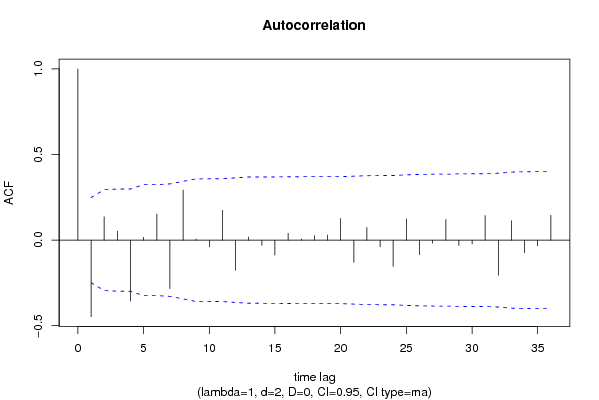
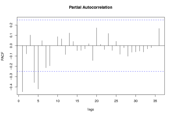
Title produced by software

(Partial) Autocorrelation Function

Date of computation

Thu, 26 Nov 2009 06:00:19 -0700

Cite this page as follows

Statistical Computations at FreeStatistics.org, Office for Research Development and Education, URL https://freestatistics.org/blog/index.php?v=date/2009/Nov/26/t1259240493kynrfxy77dhkj93.htm/, Retrieved Sun, 28 Apr 2024 18:55:14 +0000

Statistical Computations at FreeStatistics.org, Office for Research Development and Education, URL https://freestatistics.org/blog/index.php?pk=59904, Retrieved Sun, 28 Apr 2024 18:55:14 +0000

QR Codes:

Paste this QR Code to cite your computation.

Original text written by user:

IsPrivate?

No (this computation is public)

User-defined keywords

Estimated Impact

118

Family? (F = Feedback message, R = changed R code, M = changed R Module, P = changed Parameters, D = changed Data)

-     [Univariate Explorative Data Analysis] [Run Sequence gebo...] [2008-12-12 13:32:37] [76963dc1903f0f612b6153510a3818cf]
- R  D  [Univariate Explorative Data Analysis] [Run Sequence gebo...] [2008-12-17 12:14:40] [76963dc1903f0f612b6153510a3818cf]
-         [Univariate Explorative Data Analysis] [Run Sequence Plot...] [2008-12-22 18:19:51] [1ce0d16c8f4225c977b42c8fa93bc163]
- RMP       [(Partial) Autocorrelation Function] [Identifying Integ...] [2009-11-22 12:19:56] [b98453cac15ba1066b407e146608df68]
-    D        [(Partial) Autocorrelation Function] [(Partial) Autocor...] [2009-11-26 09:52:43] [976efdaed7598845c859b86bc2e467ce]
-   P             [(Partial) Autocorrelation Function] [(Partial) Autocor...] [2009-11-26 13:00:19] [d45d8d97b86162be82506c3c0ea6e4a6] [Current]

Feedback Forum

Post a new message

Dataseries X:

Download CSV

Histogram

Boxplots

1.4
1
-0.8
-2.9
-0.7
-0.7
1.5
3
3.2
3.1
3.9
1
1.3
0.8
1.2
2.9
3.9
4.5
4.5
3.3
2
1.5
1
2.1
3
4
5.1
4.5
4.2
3.3
2.7
1.8
1.4
0.5
-0.4
0.8
0.7
1.9
2
1.1
0.9
0.4
0.7
2.1
2.8
3.9
3.5
2
2
1.5
2.5
3.1
2.7
2.8
2.5
3
3.2
2.8
2.4
2
1.8
1.1
-1.5
-3.7

Summary of computational transaction
Raw Input	view raw input (R code)
Raw Output	view raw output of R engine
Computing time	1 seconds
R Server	'Gwilym Jenkins' @ 72.249.127.135

\begin{tabular}{lllllllll}
\hline
Summary of computational transaction \tabularnewline
Raw Input & view raw input (R code)  \tabularnewline
Raw Output & view raw output of R engine  \tabularnewline
Computing time & 1 seconds \tabularnewline
R Server & 'Gwilym Jenkins' @ 72.249.127.135 \tabularnewline
\hline
\end{tabular}
%Source: https://freestatistics.org/blog/index.php?pk=59904&T=0

[TABLE]
[ROW][C]Summary of computational transaction[/C][/ROW]
[ROW][C]Raw Input[/C][C]view raw input (R code) [/C][/ROW]
[ROW][C]Raw Output[/C][C]view raw output of R engine [/C][/ROW]
[ROW][C]Computing time[/C][C]1 seconds[/C][/ROW]
[ROW][C]R Server[/C][C]'Gwilym Jenkins' @ 72.249.127.135[/C][/ROW]
[/TABLE]
Source: https://freestatistics.org/blog/index.php?pk=59904&T=0

Globally Unique Identifier (entire table): ba.freestatistics.org/blog/index.php?pk=59904&T=0

As an alternative you can also use a QR Code:

The GUIDs for individual cells are displayed in the table below:

Summary of computational transaction
Raw Input	view raw input (R code)
Raw Output	view raw output of R engine
Computing time	1 seconds
R Server	'Gwilym Jenkins' @ 72.249.127.135

Autocorrelation Function
Time lag k	ACF(k)	T-STAT	P-value
1	-0.446977	-3.5195	0.000408
2	0.136018	1.071	0.144159
3	0.051982	0.4093	0.341862
4	-0.356131	-2.8042	0.003364
5	0.016624	0.1309	0.448139
6	0.152239	1.1987	0.117596
7	-0.282824	-2.227	0.014795
8	0.292866	2.306	0.012233
9	0.005919	0.0466	0.481488
10	-0.03917	-0.3084	0.379396
11	0.174271	1.3722	0.087471
12	-0.17537	-1.3809	0.086139
13	0.017809	0.1402	0.444468
14	-0.030343	-0.2389	0.405977
15	-0.086692	-0.6826	0.248697
16	0.039825	0.3136	0.377445
17	0.005956	0.0469	0.481374
18	0.026529	0.2089	0.417611
19	0.029694	0.2338	0.40795
20	0.127038	1.0003	0.160528
21	-0.129752	-1.0217	0.155454
22	0.073674	0.5801	0.281973
23	-0.038762	-0.3052	0.380613
24	-0.153724	-1.2104	0.115355
25	0.123485	0.9723	0.167334
26	-0.085142	-0.6704	0.252544
27	-0.01761	-0.1387	0.445084
28	0.120298	0.9472	0.1736
29	-0.030725	-0.2419	0.404816
30	-0.022385	-0.1763	0.430331
31	0.14341	1.1292	0.13158
32	-0.205541	-1.6184	0.055323
33	0.113706	0.8953	0.187039
34	-0.073925	-0.5821	0.281311
35	-0.033194	-0.2614	0.397335
36	0.146097	1.1504	0.127205

\begin{tabular}{lllllllll}
\hline
Autocorrelation Function \tabularnewline
Time lag k & ACF(k) & T-STAT & P-value \tabularnewline
1 & -0.446977 & -3.5195 & 0.000408 \tabularnewline
2 & 0.136018 & 1.071 & 0.144159 \tabularnewline
3 & 0.051982 & 0.4093 & 0.341862 \tabularnewline
4 & -0.356131 & -2.8042 & 0.003364 \tabularnewline
5 & 0.016624 & 0.1309 & 0.448139 \tabularnewline
6 & 0.152239 & 1.1987 & 0.117596 \tabularnewline
7 & -0.282824 & -2.227 & 0.014795 \tabularnewline
8 & 0.292866 & 2.306 & 0.012233 \tabularnewline
9 & 0.005919 & 0.0466 & 0.481488 \tabularnewline
10 & -0.03917 & -0.3084 & 0.379396 \tabularnewline
11 & 0.174271 & 1.3722 & 0.087471 \tabularnewline
12 & -0.17537 & -1.3809 & 0.086139 \tabularnewline
13 & 0.017809 & 0.1402 & 0.444468 \tabularnewline
14 & -0.030343 & -0.2389 & 0.405977 \tabularnewline
15 & -0.086692 & -0.6826 & 0.248697 \tabularnewline
16 & 0.039825 & 0.3136 & 0.377445 \tabularnewline
17 & 0.005956 & 0.0469 & 0.481374 \tabularnewline
18 & 0.026529 & 0.2089 & 0.417611 \tabularnewline
19 & 0.029694 & 0.2338 & 0.40795 \tabularnewline
20 & 0.127038 & 1.0003 & 0.160528 \tabularnewline
21 & -0.129752 & -1.0217 & 0.155454 \tabularnewline
22 & 0.073674 & 0.5801 & 0.281973 \tabularnewline
23 & -0.038762 & -0.3052 & 0.380613 \tabularnewline
24 & -0.153724 & -1.2104 & 0.115355 \tabularnewline
25 & 0.123485 & 0.9723 & 0.167334 \tabularnewline
26 & -0.085142 & -0.6704 & 0.252544 \tabularnewline
27 & -0.01761 & -0.1387 & 0.445084 \tabularnewline
28 & 0.120298 & 0.9472 & 0.1736 \tabularnewline
29 & -0.030725 & -0.2419 & 0.404816 \tabularnewline
30 & -0.022385 & -0.1763 & 0.430331 \tabularnewline
31 & 0.14341 & 1.1292 & 0.13158 \tabularnewline
32 & -0.205541 & -1.6184 & 0.055323 \tabularnewline
33 & 0.113706 & 0.8953 & 0.187039 \tabularnewline
34 & -0.073925 & -0.5821 & 0.281311 \tabularnewline
35 & -0.033194 & -0.2614 & 0.397335 \tabularnewline
36 & 0.146097 & 1.1504 & 0.127205 \tabularnewline
\hline
\end{tabular}
%Source: https://freestatistics.org/blog/index.php?pk=59904&T=1

[TABLE]
[ROW][C]Autocorrelation Function[/C][/ROW]
[ROW][C]Time lag k[/C][C]ACF(k)[/C][C]T-STAT[/C][C]P-value[/C][/ROW]
[ROW][C]1[/C][C]-0.446977[/C][C]-3.5195[/C][C]0.000408[/C][/ROW]
[ROW][C]2[/C][C]0.136018[/C][C]1.071[/C][C]0.144159[/C][/ROW]
[ROW][C]3[/C][C]0.051982[/C][C]0.4093[/C][C]0.341862[/C][/ROW]
[ROW][C]4[/C][C]-0.356131[/C][C]-2.8042[/C][C]0.003364[/C][/ROW]
[ROW][C]5[/C][C]0.016624[/C][C]0.1309[/C][C]0.448139[/C][/ROW]
[ROW][C]6[/C][C]0.152239[/C][C]1.1987[/C][C]0.117596[/C][/ROW]
[ROW][C]7[/C][C]-0.282824[/C][C]-2.227[/C][C]0.014795[/C][/ROW]
[ROW][C]8[/C][C]0.292866[/C][C]2.306[/C][C]0.012233[/C][/ROW]
[ROW][C]9[/C][C]0.005919[/C][C]0.0466[/C][C]0.481488[/C][/ROW]
[ROW][C]10[/C][C]-0.03917[/C][C]-0.3084[/C][C]0.379396[/C][/ROW]
[ROW][C]11[/C][C]0.174271[/C][C]1.3722[/C][C]0.087471[/C][/ROW]
[ROW][C]12[/C][C]-0.17537[/C][C]-1.3809[/C][C]0.086139[/C][/ROW]
[ROW][C]13[/C][C]0.017809[/C][C]0.1402[/C][C]0.444468[/C][/ROW]
[ROW][C]14[/C][C]-0.030343[/C][C]-0.2389[/C][C]0.405977[/C][/ROW]
[ROW][C]15[/C][C]-0.086692[/C][C]-0.6826[/C][C]0.248697[/C][/ROW]
[ROW][C]16[/C][C]0.039825[/C][C]0.3136[/C][C]0.377445[/C][/ROW]
[ROW][C]17[/C][C]0.005956[/C][C]0.0469[/C][C]0.481374[/C][/ROW]
[ROW][C]18[/C][C]0.026529[/C][C]0.2089[/C][C]0.417611[/C][/ROW]
[ROW][C]19[/C][C]0.029694[/C][C]0.2338[/C][C]0.40795[/C][/ROW]
[ROW][C]20[/C][C]0.127038[/C][C]1.0003[/C][C]0.160528[/C][/ROW]
[ROW][C]21[/C][C]-0.129752[/C][C]-1.0217[/C][C]0.155454[/C][/ROW]
[ROW][C]22[/C][C]0.073674[/C][C]0.5801[/C][C]0.281973[/C][/ROW]
[ROW][C]23[/C][C]-0.038762[/C][C]-0.3052[/C][C]0.380613[/C][/ROW]
[ROW][C]24[/C][C]-0.153724[/C][C]-1.2104[/C][C]0.115355[/C][/ROW]
[ROW][C]25[/C][C]0.123485[/C][C]0.9723[/C][C]0.167334[/C][/ROW]
[ROW][C]26[/C][C]-0.085142[/C][C]-0.6704[/C][C]0.252544[/C][/ROW]
[ROW][C]27[/C][C]-0.01761[/C][C]-0.1387[/C][C]0.445084[/C][/ROW]
[ROW][C]28[/C][C]0.120298[/C][C]0.9472[/C][C]0.1736[/C][/ROW]
[ROW][C]29[/C][C]-0.030725[/C][C]-0.2419[/C][C]0.404816[/C][/ROW]
[ROW][C]30[/C][C]-0.022385[/C][C]-0.1763[/C][C]0.430331[/C][/ROW]
[ROW][C]31[/C][C]0.14341[/C][C]1.1292[/C][C]0.13158[/C][/ROW]
[ROW][C]32[/C][C]-0.205541[/C][C]-1.6184[/C][C]0.055323[/C][/ROW]
[ROW][C]33[/C][C]0.113706[/C][C]0.8953[/C][C]0.187039[/C][/ROW]
[ROW][C]34[/C][C]-0.073925[/C][C]-0.5821[/C][C]0.281311[/C][/ROW]
[ROW][C]35[/C][C]-0.033194[/C][C]-0.2614[/C][C]0.397335[/C][/ROW]
[ROW][C]36[/C][C]0.146097[/C][C]1.1504[/C][C]0.127205[/C][/ROW]
[/TABLE]
Source: https://freestatistics.org/blog/index.php?pk=59904&T=1

Globally Unique Identifier (entire table): ba.freestatistics.org/blog/index.php?pk=59904&T=1

As an alternative you can also use a QR Code:

The GUIDs for individual cells are displayed in the table below:

Autocorrelation Function
Time lag k	ACF(k)	T-STAT	P-value
1	-0.446977	-3.5195	0.000408
2	0.136018	1.071	0.144159
3	0.051982	0.4093	0.341862
4	-0.356131	-2.8042	0.003364
5	0.016624	0.1309	0.448139
6	0.152239	1.1987	0.117596
7	-0.282824	-2.227	0.014795
8	0.292866	2.306	0.012233
9	0.005919	0.0466	0.481488
10	-0.03917	-0.3084	0.379396
11	0.174271	1.3722	0.087471
12	-0.17537	-1.3809	0.086139
13	0.017809	0.1402	0.444468
14	-0.030343	-0.2389	0.405977
15	-0.086692	-0.6826	0.248697
16	0.039825	0.3136	0.377445
17	0.005956	0.0469	0.481374
18	0.026529	0.2089	0.417611
19	0.029694	0.2338	0.40795
20	0.127038	1.0003	0.160528
21	-0.129752	-1.0217	0.155454
22	0.073674	0.5801	0.281973
23	-0.038762	-0.3052	0.380613
24	-0.153724	-1.2104	0.115355
25	0.123485	0.9723	0.167334
26	-0.085142	-0.6704	0.252544
27	-0.01761	-0.1387	0.445084
28	0.120298	0.9472	0.1736
29	-0.030725	-0.2419	0.404816
30	-0.022385	-0.1763	0.430331
31	0.14341	1.1292	0.13158
32	-0.205541	-1.6184	0.055323
33	0.113706	0.8953	0.187039
34	-0.073925	-0.5821	0.281311
35	-0.033194	-0.2614	0.397335
36	0.146097	1.1504	0.127205

Partial Autocorrelation Function
Time lag k	PACF(k)	T-STAT	P-value
1	-0.446977	-3.5195	0.000408
2	-0.079693	-0.6275	0.266317
3	0.103132	0.8121	0.209931
4	-0.357588	-2.8156	0.003259
5	-0.419572	-3.3037	0.000794
6	0.049555	0.3902	0.348864
7	-0.214421	-1.6884	0.048184
8	-0.195081	-1.5361	0.064805
9	0.000175	0.0014	0.499454
10	0.087625	0.69	0.246397
11	0.067043	0.5279	0.299728
12	-0.085713	-0.6749	0.251123
13	0.123395	0.9716	0.16751
14	0.041798	0.3291	0.371589
15	-0.048132	-0.379	0.352994
16	-0.046078	-0.3628	0.358989
17	-0.030823	-0.2427	0.40452
18	0.019492	0.1535	0.439258
19	-0.14387	-1.1328	0.130823
20	0.173148	1.3634	0.088849
21	0.013176	0.1037	0.458853
22	-0.037592	-0.296	0.38411
23	0.119113	0.9379	0.175968
24	-0.046407	-0.3654	0.358026
25	0.04288	0.3376	0.368388
26	-0.083113	-0.6544	0.257626
27	-0.020493	-0.1614	0.436168
28	-0.102587	-0.8078	0.211154
29	-0.063581	-0.5006	0.3092
30	-0.060358	-0.4753	0.318135
31	-0.052488	-0.4133	0.340409
32	-0.061076	-0.4809	0.316135
33	-0.031477	-0.2478	0.402536
34	-0.019401	-0.1528	0.439539
35	-0.000321	-0.0025	0.498995
36	0.166981	1.3148	0.096709

\begin{tabular}{lllllllll}
\hline
Partial Autocorrelation Function \tabularnewline
Time lag k & PACF(k) & T-STAT & P-value \tabularnewline
1 & -0.446977 & -3.5195 & 0.000408 \tabularnewline
2 & -0.079693 & -0.6275 & 0.266317 \tabularnewline
3 & 0.103132 & 0.8121 & 0.209931 \tabularnewline
4 & -0.357588 & -2.8156 & 0.003259 \tabularnewline
5 & -0.419572 & -3.3037 & 0.000794 \tabularnewline
6 & 0.049555 & 0.3902 & 0.348864 \tabularnewline
7 & -0.214421 & -1.6884 & 0.048184 \tabularnewline
8 & -0.195081 & -1.5361 & 0.064805 \tabularnewline
9 & 0.000175 & 0.0014 & 0.499454 \tabularnewline
10 & 0.087625 & 0.69 & 0.246397 \tabularnewline
11 & 0.067043 & 0.5279 & 0.299728 \tabularnewline
12 & -0.085713 & -0.6749 & 0.251123 \tabularnewline
13 & 0.123395 & 0.9716 & 0.16751 \tabularnewline
14 & 0.041798 & 0.3291 & 0.371589 \tabularnewline
15 & -0.048132 & -0.379 & 0.352994 \tabularnewline
16 & -0.046078 & -0.3628 & 0.358989 \tabularnewline
17 & -0.030823 & -0.2427 & 0.40452 \tabularnewline
18 & 0.019492 & 0.1535 & 0.439258 \tabularnewline
19 & -0.14387 & -1.1328 & 0.130823 \tabularnewline
20 & 0.173148 & 1.3634 & 0.088849 \tabularnewline
21 & 0.013176 & 0.1037 & 0.458853 \tabularnewline
22 & -0.037592 & -0.296 & 0.38411 \tabularnewline
23 & 0.119113 & 0.9379 & 0.175968 \tabularnewline
24 & -0.046407 & -0.3654 & 0.358026 \tabularnewline
25 & 0.04288 & 0.3376 & 0.368388 \tabularnewline
26 & -0.083113 & -0.6544 & 0.257626 \tabularnewline
27 & -0.020493 & -0.1614 & 0.436168 \tabularnewline
28 & -0.102587 & -0.8078 & 0.211154 \tabularnewline
29 & -0.063581 & -0.5006 & 0.3092 \tabularnewline
30 & -0.060358 & -0.4753 & 0.318135 \tabularnewline
31 & -0.052488 & -0.4133 & 0.340409 \tabularnewline
32 & -0.061076 & -0.4809 & 0.316135 \tabularnewline
33 & -0.031477 & -0.2478 & 0.402536 \tabularnewline
34 & -0.019401 & -0.1528 & 0.439539 \tabularnewline
35 & -0.000321 & -0.0025 & 0.498995 \tabularnewline
36 & 0.166981 & 1.3148 & 0.096709 \tabularnewline
\hline
\end{tabular}
%Source: https://freestatistics.org/blog/index.php?pk=59904&T=2

[TABLE]
[ROW][C]Partial Autocorrelation Function[/C][/ROW]
[ROW][C]Time lag k[/C][C]PACF(k)[/C][C]T-STAT[/C][C]P-value[/C][/ROW]
[ROW][C]1[/C][C]-0.446977[/C][C]-3.5195[/C][C]0.000408[/C][/ROW]
[ROW][C]2[/C][C]-0.079693[/C][C]-0.6275[/C][C]0.266317[/C][/ROW]
[ROW][C]3[/C][C]0.103132[/C][C]0.8121[/C][C]0.209931[/C][/ROW]
[ROW][C]4[/C][C]-0.357588[/C][C]-2.8156[/C][C]0.003259[/C][/ROW]
[ROW][C]5[/C][C]-0.419572[/C][C]-3.3037[/C][C]0.000794[/C][/ROW]
[ROW][C]6[/C][C]0.049555[/C][C]0.3902[/C][C]0.348864[/C][/ROW]
[ROW][C]7[/C][C]-0.214421[/C][C]-1.6884[/C][C]0.048184[/C][/ROW]
[ROW][C]8[/C][C]-0.195081[/C][C]-1.5361[/C][C]0.064805[/C][/ROW]
[ROW][C]9[/C][C]0.000175[/C][C]0.0014[/C][C]0.499454[/C][/ROW]
[ROW][C]10[/C][C]0.087625[/C][C]0.69[/C][C]0.246397[/C][/ROW]
[ROW][C]11[/C][C]0.067043[/C][C]0.5279[/C][C]0.299728[/C][/ROW]
[ROW][C]12[/C][C]-0.085713[/C][C]-0.6749[/C][C]0.251123[/C][/ROW]
[ROW][C]13[/C][C]0.123395[/C][C]0.9716[/C][C]0.16751[/C][/ROW]
[ROW][C]14[/C][C]0.041798[/C][C]0.3291[/C][C]0.371589[/C][/ROW]
[ROW][C]15[/C][C]-0.048132[/C][C]-0.379[/C][C]0.352994[/C][/ROW]
[ROW][C]16[/C][C]-0.046078[/C][C]-0.3628[/C][C]0.358989[/C][/ROW]
[ROW][C]17[/C][C]-0.030823[/C][C]-0.2427[/C][C]0.40452[/C][/ROW]
[ROW][C]18[/C][C]0.019492[/C][C]0.1535[/C][C]0.439258[/C][/ROW]
[ROW][C]19[/C][C]-0.14387[/C][C]-1.1328[/C][C]0.130823[/C][/ROW]
[ROW][C]20[/C][C]0.173148[/C][C]1.3634[/C][C]0.088849[/C][/ROW]
[ROW][C]21[/C][C]0.013176[/C][C]0.1037[/C][C]0.458853[/C][/ROW]
[ROW][C]22[/C][C]-0.037592[/C][C]-0.296[/C][C]0.38411[/C][/ROW]
[ROW][C]23[/C][C]0.119113[/C][C]0.9379[/C][C]0.175968[/C][/ROW]
[ROW][C]24[/C][C]-0.046407[/C][C]-0.3654[/C][C]0.358026[/C][/ROW]
[ROW][C]25[/C][C]0.04288[/C][C]0.3376[/C][C]0.368388[/C][/ROW]
[ROW][C]26[/C][C]-0.083113[/C][C]-0.6544[/C][C]0.257626[/C][/ROW]
[ROW][C]27[/C][C]-0.020493[/C][C]-0.1614[/C][C]0.436168[/C][/ROW]
[ROW][C]28[/C][C]-0.102587[/C][C]-0.8078[/C][C]0.211154[/C][/ROW]
[ROW][C]29[/C][C]-0.063581[/C][C]-0.5006[/C][C]0.3092[/C][/ROW]
[ROW][C]30[/C][C]-0.060358[/C][C]-0.4753[/C][C]0.318135[/C][/ROW]
[ROW][C]31[/C][C]-0.052488[/C][C]-0.4133[/C][C]0.340409[/C][/ROW]
[ROW][C]32[/C][C]-0.061076[/C][C]-0.4809[/C][C]0.316135[/C][/ROW]
[ROW][C]33[/C][C]-0.031477[/C][C]-0.2478[/C][C]0.402536[/C][/ROW]
[ROW][C]34[/C][C]-0.019401[/C][C]-0.1528[/C][C]0.439539[/C][/ROW]
[ROW][C]35[/C][C]-0.000321[/C][C]-0.0025[/C][C]0.498995[/C][/ROW]
[ROW][C]36[/C][C]0.166981[/C][C]1.3148[/C][C]0.096709[/C][/ROW]
[/TABLE]
Source: https://freestatistics.org/blog/index.php?pk=59904&T=2

Globally Unique Identifier (entire table): ba.freestatistics.org/blog/index.php?pk=59904&T=2

As an alternative you can also use a QR Code:

The GUIDs for individual cells are displayed in the table below:

Partial Autocorrelation Function
Time lag k	PACF(k)	T-STAT	P-value
1	-0.446977	-3.5195	0.000408
2	-0.079693	-0.6275	0.266317
3	0.103132	0.8121	0.209931
4	-0.357588	-2.8156	0.003259
5	-0.419572	-3.3037	0.000794
6	0.049555	0.3902	0.348864
7	-0.214421	-1.6884	0.048184
8	-0.195081	-1.5361	0.064805
9	0.000175	0.0014	0.499454
10	0.087625	0.69	0.246397
11	0.067043	0.5279	0.299728
12	-0.085713	-0.6749	0.251123
13	0.123395	0.9716	0.16751
14	0.041798	0.3291	0.371589
15	-0.048132	-0.379	0.352994
16	-0.046078	-0.3628	0.358989
17	-0.030823	-0.2427	0.40452
18	0.019492	0.1535	0.439258
19	-0.14387	-1.1328	0.130823
20	0.173148	1.3634	0.088849
21	0.013176	0.1037	0.458853
22	-0.037592	-0.296	0.38411
23	0.119113	0.9379	0.175968
24	-0.046407	-0.3654	0.358026
25	0.04288	0.3376	0.368388
26	-0.083113	-0.6544	0.257626
27	-0.020493	-0.1614	0.436168
28	-0.102587	-0.8078	0.211154
29	-0.063581	-0.5006	0.3092
30	-0.060358	-0.4753	0.318135
31	-0.052488	-0.4133	0.340409
32	-0.061076	-0.4809	0.316135
33	-0.031477	-0.2478	0.402536
34	-0.019401	-0.1528	0.439539
35	-0.000321	-0.0025	0.498995
36	0.166981	1.3148	0.096709

Figure 1

PNG link

Postscript link

PDF link

Figure 2

PNG link

Postscript link

PDF link

Parameters (Session):

par1 = 36 ; par2 = 1 ; par3 = 2 ; par4 = 0 ; par5 = 12 ; par6 = MA ; par7 = 0.95 ;

Parameters (R input):

par1 = 36 ; par2 = 1 ; par3 = 2 ; par4 = 0 ; par5 = 12 ; par6 = MA ; par7 = 0.95 ;

R code (references can be found in the software module):

if (par1 == 'Default') {
par1 = 10*log10(length(x))
} else {
par1 <- as.numeric(par1)
}
par2 <- as.numeric(par2)
par3 <- as.numeric(par3)
par4 <- as.numeric(par4)
par5 <- as.numeric(par5)
if (par6 == 'White Noise') par6 <- 'white' else par6 <- 'ma'
par7 <- as.numeric(par7)
if (par2 == 0) {
x <- log(x)
} else {
x <- (x ^ par2 - 1) / par2
}
if (par3 > 0) x <- diff(x,lag=1,difference=par3)
if (par4 > 0) x <- diff(x,lag=par5,difference=par4)
bitmap(file='pic1.png')
racf <- acf(x, par1, main='Autocorrelation', xlab='time lag', ylab='ACF', ci.type=par6, ci=par7, sub=paste('(lambda=',par2,', d=',par3,', D=',par4,', CI=', par7, ', CI type=',par6,')',sep=''))
dev.off()
bitmap(file='pic2.png')
rpacf <- pacf(x,par1,main='Partial Autocorrelation',xlab='lags',ylab='PACF')
dev.off()
(myacf <- c(racf$acf))
(mypacf <- c(rpacf$acf))
lengthx <- length(x)
sqrtn <- sqrt(lengthx)
load(file='createtable')
a<-table.start()
a<-table.row.start(a)
a<-table.element(a,'Autocorrelation Function',4,TRUE)
a<-table.row.end(a)
a<-table.row.start(a)
a<-table.element(a,'Time lag k',header=TRUE)
a<-table.element(a,hyperlink('basics.htm','ACF(k)','click here for more information about the Autocorrelation Function'),header=TRUE)
a<-table.element(a,'T-STAT',header=TRUE)
a<-table.element(a,'P-value',header=TRUE)
a<-table.row.end(a)
for (i in 2:(par1+1)) {
a<-table.row.start(a)
a<-table.element(a,i-1,header=TRUE)
a<-table.element(a,round(myacf[i],6))
mytstat <- myacf[i]*sqrtn
a<-table.element(a,round(mytstat,4))
a<-table.element(a,round(1-pt(abs(mytstat),lengthx),6))
a<-table.row.end(a)
}
a<-table.end(a)
table.save(a,file='mytable.tab')
a<-table.start()
a<-table.row.start(a)
a<-table.element(a,'Partial Autocorrelation Function',4,TRUE)
a<-table.row.end(a)
a<-table.row.start(a)
a<-table.element(a,'Time lag k',header=TRUE)
a<-table.element(a,hyperlink('basics.htm','PACF(k)','click here for more information about the Partial Autocorrelation Function'),header=TRUE)
a<-table.element(a,'T-STAT',header=TRUE)
a<-table.element(a,'P-value',header=TRUE)
a<-table.row.end(a)
for (i in 1:par1) {
a<-table.row.start(a)
a<-table.element(a,i,header=TRUE)
a<-table.element(a,round(mypacf[i],6))
mytstat <- mypacf[i]*sqrtn
a<-table.element(a,round(mytstat,4))
a<-table.element(a,round(1-pt(abs(mytstat),lengthx),6))
a<-table.row.end(a)
}
a<-table.end(a)
table.save(a,file='mytable1.tab')

Free Statistics

Description of Statistical Computation

Tree of Dependent Computations

Dataset

Tables (Output of Computation)

Figures (Output of Computation)

Input Parameters & R Code