Repository of Reproducible Computations

Free Statistics

of Irreproducible Research!

Author's title

Author

*The author of this computation has been verified*

R Software Module

rwasp_autocorrelation.wasp

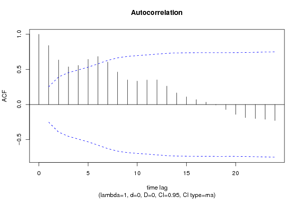
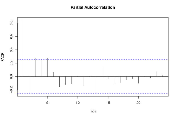
Title produced by software

(Partial) Autocorrelation Function

Date of computation

Thu, 26 Nov 2009 07:51:36 -0700

Cite this page as follows

Statistical Computations at FreeStatistics.org, Office for Research Development and Education, URL https://freestatistics.org/blog/index.php?v=date/2009/Nov/26/t1259247309y4bxhba47kbmzyq.htm/, Retrieved Mon, 29 Apr 2024 04:15:10 +0000

Statistical Computations at FreeStatistics.org, Office for Research Development and Education, URL https://freestatistics.org/blog/index.php?pk=60054, Retrieved Mon, 29 Apr 2024 04:15:10 +0000

QR Codes:

Paste this QR Code to cite your computation.

Original text written by user:

IsPrivate?

No (this computation is public)

User-defined keywords

Estimated Impact

130

Family? (F = Feedback message, R = changed R code, M = changed R Module, P = changed Parameters, D = changed Data)

-     [Univariate Explorative Data Analysis] [Run Sequence gebo...] [2008-12-12 13:32:37] [76963dc1903f0f612b6153510a3818cf]
- R  D  [Univariate Explorative Data Analysis] [Run Sequence gebo...] [2008-12-17 12:14:40] [76963dc1903f0f612b6153510a3818cf]
-         [Univariate Explorative Data Analysis] [Run Sequence Plot...] [2008-12-22 18:19:51] [1ce0d16c8f4225c977b42c8fa93bc163]
- RMP       [(Partial) Autocorrelation Function] [Identifying Integ...] [2009-11-22 12:16:10] [b98453cac15ba1066b407e146608df68]
-    D        [(Partial) Autocorrelation Function] [] [2009-11-26 09:49:31] [d181e5359f7da6c8509e4702d1229fb0]
-   PD            [(Partial) Autocorrelation Function] [] [2009-11-26 14:51:36] [5858ea01c9bd81debbf921a11363ad90] [Current]
- RMPD              [Variance Reduction Matrix] [] [2009-12-21 12:47:46] [8f79fe502d085bc4aad43092067387d5] 

Feedback Forum

Post a new message

Dataseries X:

Download CSV

Histogram

Boxplots

Summary of computational transaction
Raw Input	view raw input (R code)
Raw Output	view raw output of R engine
Computing time	1 seconds
R Server	'Gwilym Jenkins' @ 72.249.127.135

\begin{tabular}{lllllllll}
\hline
Summary of computational transaction \tabularnewline
Raw Input & view raw input (R code)  \tabularnewline
Raw Output & view raw output of R engine  \tabularnewline
Computing time & 1 seconds \tabularnewline
R Server & 'Gwilym Jenkins' @ 72.249.127.135 \tabularnewline
\hline
\end{tabular}
%Source: https://freestatistics.org/blog/index.php?pk=60054&T=0

[TABLE]
[ROW][C]Summary of computational transaction[/C][/ROW]
[ROW][C]Raw Input[/C][C]view raw input (R code) [/C][/ROW]
[ROW][C]Raw Output[/C][C]view raw output of R engine [/C][/ROW]
[ROW][C]Computing time[/C][C]1 seconds[/C][/ROW]
[ROW][C]R Server[/C][C]'Gwilym Jenkins' @ 72.249.127.135[/C][/ROW]
[/TABLE]
Source: https://freestatistics.org/blog/index.php?pk=60054&T=0

Globally Unique Identifier (entire table): ba.freestatistics.org/blog/index.php?pk=60054&T=0

As an alternative you can also use a QR Code:

The GUIDs for individual cells are displayed in the table below:

Summary of computational transaction
Raw Input	view raw input (R code)
Raw Output	view raw output of R engine
Computing time	1 seconds
R Server	'Gwilym Jenkins' @ 72.249.127.135

Autocorrelation Function
Time lag k	ACF(k)	T-STAT	P-value
1	0.840257	6.5086	0
2	0.635155	4.9199	4e-06
3	0.536466	4.1555	5.2e-05
4	0.556973	4.3143	3e-05
5	0.642806	4.9792	3e-06
6	0.684094	5.299	1e-06
7	0.604583	4.6831	8e-06
8	0.462295	3.5809	0.000343
9	0.351059	2.7193	0.004272
10	0.333693	2.5848	0.006097
11	0.34899	2.7033	0.004459
12	0.351702	2.7243	0.004215
13	0.261906	2.0287	0.023466
14	0.165671	1.2833	0.102164
15	0.108441	0.84	0.202126
16	0.069541	0.5387	0.296056
17	0.034745	0.2691	0.394375
18	-0.007022	-0.0544	0.478402
19	-0.071599	-0.5546	0.290613
20	-0.141024	-1.0924	0.139519
21	-0.186761	-1.4466	0.076601
22	-0.200105	-1.55	0.0632
23	-0.211276	-1.6365	0.053481
24	-0.228416	-1.7693	0.040962

\begin{tabular}{lllllllll}
\hline
Autocorrelation Function \tabularnewline
Time lag k & ACF(k) & T-STAT & P-value \tabularnewline
1 & 0.840257 & 6.5086 & 0 \tabularnewline
2 & 0.635155 & 4.9199 & 4e-06 \tabularnewline
3 & 0.536466 & 4.1555 & 5.2e-05 \tabularnewline
4 & 0.556973 & 4.3143 & 3e-05 \tabularnewline
5 & 0.642806 & 4.9792 & 3e-06 \tabularnewline
6 & 0.684094 & 5.299 & 1e-06 \tabularnewline
7 & 0.604583 & 4.6831 & 8e-06 \tabularnewline
8 & 0.462295 & 3.5809 & 0.000343 \tabularnewline
9 & 0.351059 & 2.7193 & 0.004272 \tabularnewline
10 & 0.333693 & 2.5848 & 0.006097 \tabularnewline
11 & 0.34899 & 2.7033 & 0.004459 \tabularnewline
12 & 0.351702 & 2.7243 & 0.004215 \tabularnewline
13 & 0.261906 & 2.0287 & 0.023466 \tabularnewline
14 & 0.165671 & 1.2833 & 0.102164 \tabularnewline
15 & 0.108441 & 0.84 & 0.202126 \tabularnewline
16 & 0.069541 & 0.5387 & 0.296056 \tabularnewline
17 & 0.034745 & 0.2691 & 0.394375 \tabularnewline
18 & -0.007022 & -0.0544 & 0.478402 \tabularnewline
19 & -0.071599 & -0.5546 & 0.290613 \tabularnewline
20 & -0.141024 & -1.0924 & 0.139519 \tabularnewline
21 & -0.186761 & -1.4466 & 0.076601 \tabularnewline
22 & -0.200105 & -1.55 & 0.0632 \tabularnewline
23 & -0.211276 & -1.6365 & 0.053481 \tabularnewline
24 & -0.228416 & -1.7693 & 0.040962 \tabularnewline
\hline
\end{tabular}
%Source: https://freestatistics.org/blog/index.php?pk=60054&T=1

[TABLE]
[ROW][C]Autocorrelation Function[/C][/ROW]
[ROW][C]Time lag k[/C][C]ACF(k)[/C][C]T-STAT[/C][C]P-value[/C][/ROW]
[ROW][C]1[/C][C]0.840257[/C][C]6.5086[/C][C]0[/C][/ROW]
[ROW][C]2[/C][C]0.635155[/C][C]4.9199[/C][C]4e-06[/C][/ROW]
[ROW][C]3[/C][C]0.536466[/C][C]4.1555[/C][C]5.2e-05[/C][/ROW]
[ROW][C]4[/C][C]0.556973[/C][C]4.3143[/C][C]3e-05[/C][/ROW]
[ROW][C]5[/C][C]0.642806[/C][C]4.9792[/C][C]3e-06[/C][/ROW]
[ROW][C]6[/C][C]0.684094[/C][C]5.299[/C][C]1e-06[/C][/ROW]
[ROW][C]7[/C][C]0.604583[/C][C]4.6831[/C][C]8e-06[/C][/ROW]
[ROW][C]8[/C][C]0.462295[/C][C]3.5809[/C][C]0.000343[/C][/ROW]
[ROW][C]9[/C][C]0.351059[/C][C]2.7193[/C][C]0.004272[/C][/ROW]
[ROW][C]10[/C][C]0.333693[/C][C]2.5848[/C][C]0.006097[/C][/ROW]
[ROW][C]11[/C][C]0.34899[/C][C]2.7033[/C][C]0.004459[/C][/ROW]
[ROW][C]12[/C][C]0.351702[/C][C]2.7243[/C][C]0.004215[/C][/ROW]
[ROW][C]13[/C][C]0.261906[/C][C]2.0287[/C][C]0.023466[/C][/ROW]
[ROW][C]14[/C][C]0.165671[/C][C]1.2833[/C][C]0.102164[/C][/ROW]
[ROW][C]15[/C][C]0.108441[/C][C]0.84[/C][C]0.202126[/C][/ROW]
[ROW][C]16[/C][C]0.069541[/C][C]0.5387[/C][C]0.296056[/C][/ROW]
[ROW][C]17[/C][C]0.034745[/C][C]0.2691[/C][C]0.394375[/C][/ROW]
[ROW][C]18[/C][C]-0.007022[/C][C]-0.0544[/C][C]0.478402[/C][/ROW]
[ROW][C]19[/C][C]-0.071599[/C][C]-0.5546[/C][C]0.290613[/C][/ROW]
[ROW][C]20[/C][C]-0.141024[/C][C]-1.0924[/C][C]0.139519[/C][/ROW]
[ROW][C]21[/C][C]-0.186761[/C][C]-1.4466[/C][C]0.076601[/C][/ROW]
[ROW][C]22[/C][C]-0.200105[/C][C]-1.55[/C][C]0.0632[/C][/ROW]
[ROW][C]23[/C][C]-0.211276[/C][C]-1.6365[/C][C]0.053481[/C][/ROW]
[ROW][C]24[/C][C]-0.228416[/C][C]-1.7693[/C][C]0.040962[/C][/ROW]
[/TABLE]
Source: https://freestatistics.org/blog/index.php?pk=60054&T=1

Globally Unique Identifier (entire table): ba.freestatistics.org/blog/index.php?pk=60054&T=1

As an alternative you can also use a QR Code:

The GUIDs for individual cells are displayed in the table below:

Autocorrelation Function
Time lag k	ACF(k)	T-STAT	P-value
1	0.840257	6.5086	0
2	0.635155	4.9199	4e-06
3	0.536466	4.1555	5.2e-05
4	0.556973	4.3143	3e-05
5	0.642806	4.9792	3e-06
6	0.684094	5.299	1e-06
7	0.604583	4.6831	8e-06
8	0.462295	3.5809	0.000343
9	0.351059	2.7193	0.004272
10	0.333693	2.5848	0.006097
11	0.34899	2.7033	0.004459
12	0.351702	2.7243	0.004215
13	0.261906	2.0287	0.023466
14	0.165671	1.2833	0.102164
15	0.108441	0.84	0.202126
16	0.069541	0.5387	0.296056
17	0.034745	0.2691	0.394375
18	-0.007022	-0.0544	0.478402
19	-0.071599	-0.5546	0.290613
20	-0.141024	-1.0924	0.139519
21	-0.186761	-1.4466	0.076601
22	-0.200105	-1.55	0.0632
23	-0.211276	-1.6365	0.053481
24	-0.228416	-1.7693	0.040962

Partial Autocorrelation Function
Time lag k	PACF(k)	T-STAT	P-value
1	0.840257	6.5086	0
2	-0.241102	-1.8676	0.033354
3	0.276966	2.1454	0.01799
4	0.256478	1.9867	0.025766
5	0.272402	2.11	0.019518
6	0.063814	0.4943	0.311449
7	-0.154231	-1.1947	0.118459
8	-0.120789	-0.9356	0.176607
9	-0.110024	-0.8522	0.198734
10	0.004522	0.035	0.486087
11	-0.14232	-1.1024	0.137344
12	0.00717	0.0555	0.477948
13	-0.239592	-1.8559	0.034193
14	0.129902	1.0062	0.159176
15	-0.038045	-0.2947	0.384621
16	-0.107499	-0.8327	0.204163
17	-0.090221	-0.6988	0.243674
18	-0.050275	-0.3894	0.34917
19	-0.032191	-0.2493	0.401971
20	-0.101823	-0.7887	0.216691
21	-0.000777	-0.006	0.49761
22	-0.021013	-0.1628	0.435624
23	0.07355	0.5697	0.285498
24	0.018858	0.1461	0.442176

\begin{tabular}{lllllllll}
\hline
Partial Autocorrelation Function \tabularnewline
Time lag k & PACF(k) & T-STAT & P-value \tabularnewline
1 & 0.840257 & 6.5086 & 0 \tabularnewline
2 & -0.241102 & -1.8676 & 0.033354 \tabularnewline
3 & 0.276966 & 2.1454 & 0.01799 \tabularnewline
4 & 0.256478 & 1.9867 & 0.025766 \tabularnewline
5 & 0.272402 & 2.11 & 0.019518 \tabularnewline
6 & 0.063814 & 0.4943 & 0.311449 \tabularnewline
7 & -0.154231 & -1.1947 & 0.118459 \tabularnewline
8 & -0.120789 & -0.9356 & 0.176607 \tabularnewline
9 & -0.110024 & -0.8522 & 0.198734 \tabularnewline
10 & 0.004522 & 0.035 & 0.486087 \tabularnewline
11 & -0.14232 & -1.1024 & 0.137344 \tabularnewline
12 & 0.00717 & 0.0555 & 0.477948 \tabularnewline
13 & -0.239592 & -1.8559 & 0.034193 \tabularnewline
14 & 0.129902 & 1.0062 & 0.159176 \tabularnewline
15 & -0.038045 & -0.2947 & 0.384621 \tabularnewline
16 & -0.107499 & -0.8327 & 0.204163 \tabularnewline
17 & -0.090221 & -0.6988 & 0.243674 \tabularnewline
18 & -0.050275 & -0.3894 & 0.34917 \tabularnewline
19 & -0.032191 & -0.2493 & 0.401971 \tabularnewline
20 & -0.101823 & -0.7887 & 0.216691 \tabularnewline
21 & -0.000777 & -0.006 & 0.49761 \tabularnewline
22 & -0.021013 & -0.1628 & 0.435624 \tabularnewline
23 & 0.07355 & 0.5697 & 0.285498 \tabularnewline
24 & 0.018858 & 0.1461 & 0.442176 \tabularnewline
\hline
\end{tabular}
%Source: https://freestatistics.org/blog/index.php?pk=60054&T=2

[TABLE]
[ROW][C]Partial Autocorrelation Function[/C][/ROW]
[ROW][C]Time lag k[/C][C]PACF(k)[/C][C]T-STAT[/C][C]P-value[/C][/ROW]
[ROW][C]1[/C][C]0.840257[/C][C]6.5086[/C][C]0[/C][/ROW]
[ROW][C]2[/C][C]-0.241102[/C][C]-1.8676[/C][C]0.033354[/C][/ROW]
[ROW][C]3[/C][C]0.276966[/C][C]2.1454[/C][C]0.01799[/C][/ROW]
[ROW][C]4[/C][C]0.256478[/C][C]1.9867[/C][C]0.025766[/C][/ROW]
[ROW][C]5[/C][C]0.272402[/C][C]2.11[/C][C]0.019518[/C][/ROW]
[ROW][C]6[/C][C]0.063814[/C][C]0.4943[/C][C]0.311449[/C][/ROW]
[ROW][C]7[/C][C]-0.154231[/C][C]-1.1947[/C][C]0.118459[/C][/ROW]
[ROW][C]8[/C][C]-0.120789[/C][C]-0.9356[/C][C]0.176607[/C][/ROW]
[ROW][C]9[/C][C]-0.110024[/C][C]-0.8522[/C][C]0.198734[/C][/ROW]
[ROW][C]10[/C][C]0.004522[/C][C]0.035[/C][C]0.486087[/C][/ROW]
[ROW][C]11[/C][C]-0.14232[/C][C]-1.1024[/C][C]0.137344[/C][/ROW]
[ROW][C]12[/C][C]0.00717[/C][C]0.0555[/C][C]0.477948[/C][/ROW]
[ROW][C]13[/C][C]-0.239592[/C][C]-1.8559[/C][C]0.034193[/C][/ROW]
[ROW][C]14[/C][C]0.129902[/C][C]1.0062[/C][C]0.159176[/C][/ROW]
[ROW][C]15[/C][C]-0.038045[/C][C]-0.2947[/C][C]0.384621[/C][/ROW]
[ROW][C]16[/C][C]-0.107499[/C][C]-0.8327[/C][C]0.204163[/C][/ROW]
[ROW][C]17[/C][C]-0.090221[/C][C]-0.6988[/C][C]0.243674[/C][/ROW]
[ROW][C]18[/C][C]-0.050275[/C][C]-0.3894[/C][C]0.34917[/C][/ROW]
[ROW][C]19[/C][C]-0.032191[/C][C]-0.2493[/C][C]0.401971[/C][/ROW]
[ROW][C]20[/C][C]-0.101823[/C][C]-0.7887[/C][C]0.216691[/C][/ROW]
[ROW][C]21[/C][C]-0.000777[/C][C]-0.006[/C][C]0.49761[/C][/ROW]
[ROW][C]22[/C][C]-0.021013[/C][C]-0.1628[/C][C]0.435624[/C][/ROW]
[ROW][C]23[/C][C]0.07355[/C][C]0.5697[/C][C]0.285498[/C][/ROW]
[ROW][C]24[/C][C]0.018858[/C][C]0.1461[/C][C]0.442176[/C][/ROW]
[/TABLE]
Source: https://freestatistics.org/blog/index.php?pk=60054&T=2

Globally Unique Identifier (entire table): ba.freestatistics.org/blog/index.php?pk=60054&T=2

As an alternative you can also use a QR Code:

The GUIDs for individual cells are displayed in the table below:

Partial Autocorrelation Function
Time lag k	PACF(k)	T-STAT	P-value
1	0.840257	6.5086	0
2	-0.241102	-1.8676	0.033354
3	0.276966	2.1454	0.01799
4	0.256478	1.9867	0.025766
5	0.272402	2.11	0.019518
6	0.063814	0.4943	0.311449
7	-0.154231	-1.1947	0.118459
8	-0.120789	-0.9356	0.176607
9	-0.110024	-0.8522	0.198734
10	0.004522	0.035	0.486087
11	-0.14232	-1.1024	0.137344
12	0.00717	0.0555	0.477948
13	-0.239592	-1.8559	0.034193
14	0.129902	1.0062	0.159176
15	-0.038045	-0.2947	0.384621
16	-0.107499	-0.8327	0.204163
17	-0.090221	-0.6988	0.243674
18	-0.050275	-0.3894	0.34917
19	-0.032191	-0.2493	0.401971
20	-0.101823	-0.7887	0.216691
21	-0.000777	-0.006	0.49761
22	-0.021013	-0.1628	0.435624
23	0.07355	0.5697	0.285498
24	0.018858	0.1461	0.442176

Figure 1

PNG link

Postscript link

PDF link

Figure 2

PNG link

Postscript link

PDF link

Parameters (Session):

par1 = 24 ; par2 = 1 ; par3 = 0 ; par4 = 0 ; par5 = 12 ; par6 = MA ; par7 = 0.95 ;

Parameters (R input):

par1 = 24 ; par2 = 1 ; par3 = 0 ; par4 = 0 ; par5 = 12 ; par6 = MA ; par7 = 0.95 ;

R code (references can be found in the software module):

if (par1 == 'Default') {
par1 = 10*log10(length(x))
} else {
par1 <- as.numeric(par1)
}
par2 <- as.numeric(par2)
par3 <- as.numeric(par3)
par4 <- as.numeric(par4)
par5 <- as.numeric(par5)
if (par6 == 'White Noise') par6 <- 'white' else par6 <- 'ma'
par7 <- as.numeric(par7)
if (par2 == 0) {
x <- log(x)
} else {
x <- (x ^ par2 - 1) / par2
}
if (par3 > 0) x <- diff(x,lag=1,difference=par3)
if (par4 > 0) x <- diff(x,lag=par5,difference=par4)
bitmap(file='pic1.png')
racf <- acf(x, par1, main='Autocorrelation', xlab='time lag', ylab='ACF', ci.type=par6, ci=par7, sub=paste('(lambda=',par2,', d=',par3,', D=',par4,', CI=', par7, ', CI type=',par6,')',sep=''))
dev.off()
bitmap(file='pic2.png')
rpacf <- pacf(x,par1,main='Partial Autocorrelation',xlab='lags',ylab='PACF')
dev.off()
(myacf <- c(racf$acf))
(mypacf <- c(rpacf$acf))
lengthx <- length(x)
sqrtn <- sqrt(lengthx)
load(file='createtable')
a<-table.start()
a<-table.row.start(a)
a<-table.element(a,'Autocorrelation Function',4,TRUE)
a<-table.row.end(a)
a<-table.row.start(a)
a<-table.element(a,'Time lag k',header=TRUE)
a<-table.element(a,hyperlink('basics.htm','ACF(k)','click here for more information about the Autocorrelation Function'),header=TRUE)
a<-table.element(a,'T-STAT',header=TRUE)
a<-table.element(a,'P-value',header=TRUE)
a<-table.row.end(a)
for (i in 2:(par1+1)) {
a<-table.row.start(a)
a<-table.element(a,i-1,header=TRUE)
a<-table.element(a,round(myacf[i],6))
mytstat <- myacf[i]*sqrtn
a<-table.element(a,round(mytstat,4))
a<-table.element(a,round(1-pt(abs(mytstat),lengthx),6))
a<-table.row.end(a)
}
a<-table.end(a)
table.save(a,file='mytable.tab')
a<-table.start()
a<-table.row.start(a)
a<-table.element(a,'Partial Autocorrelation Function',4,TRUE)
a<-table.row.end(a)
a<-table.row.start(a)
a<-table.element(a,'Time lag k',header=TRUE)
a<-table.element(a,hyperlink('basics.htm','PACF(k)','click here for more information about the Partial Autocorrelation Function'),header=TRUE)
a<-table.element(a,'T-STAT',header=TRUE)
a<-table.element(a,'P-value',header=TRUE)
a<-table.row.end(a)
for (i in 1:par1) {
a<-table.row.start(a)
a<-table.element(a,i,header=TRUE)
a<-table.element(a,round(mypacf[i],6))
mytstat <- mypacf[i]*sqrtn
a<-table.element(a,round(mytstat,4))
a<-table.element(a,round(1-pt(abs(mytstat),lengthx),6))
a<-table.row.end(a)
}
a<-table.end(a)
table.save(a,file='mytable1.tab')

Free Statistics

Description of Statistical Computation

Tree of Dependent Computations

Dataset

Tables (Output of Computation)

Figures (Output of Computation)

Input Parameters & R Code