Repository of Reproducible Computations

Free Statistics

of Irreproducible Research!

Author's title

Author

*Unverified author*

R Software Module

rwasp_autocorrelation.wasp

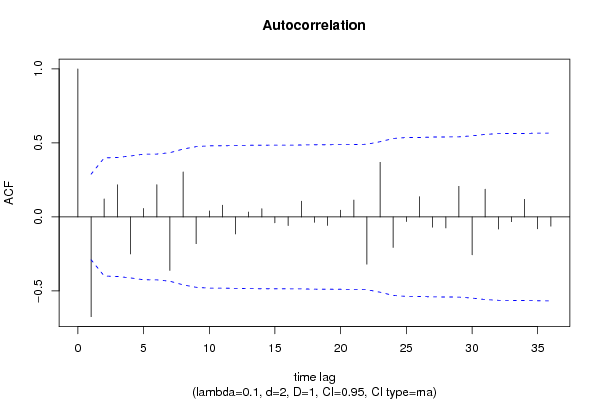
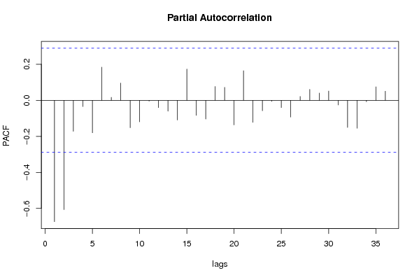
Title produced by software

(Partial) Autocorrelation Function

Date of computation

Thu, 26 Nov 2009 08:36:56 -0700

Cite this page as follows

Statistical Computations at FreeStatistics.org, Office for Research Development and Education, URL https://freestatistics.org/blog/index.php?v=date/2009/Nov/26/t12592498989yad82yh26mg1gw.htm/, Retrieved Mon, 29 Apr 2024 03:09:06 +0000

Statistical Computations at FreeStatistics.org, Office for Research Development and Education, URL https://freestatistics.org/blog/index.php?pk=60106, Retrieved Mon, 29 Apr 2024 03:09:06 +0000

QR Codes:

Paste this QR Code to cite your computation.

Original text written by user:

IsPrivate?

No (this computation is public)

User-defined keywords

Estimated Impact

125

Family? (F = Feedback message, R = changed R code, M = changed R Module, P = changed Parameters, D = changed Data)

-     [Univariate Explorative Data Analysis] [Run Sequence gebo...] [2008-12-12 13:32:37] [76963dc1903f0f612b6153510a3818cf]
- R  D  [Univariate Explorative Data Analysis] [Run Sequence gebo...] [2008-12-17 12:14:40] [76963dc1903f0f612b6153510a3818cf]
-         [Univariate Explorative Data Analysis] [Run Sequence Plot...] [2008-12-22 18:19:51] [1ce0d16c8f4225c977b42c8fa93bc163]
- RMP       [(Partial) Autocorrelation Function] [Identifying Integ...] [2009-11-22 12:26:39] [b98453cac15ba1066b407e146608df68]
-    D        [(Partial) Autocorrelation Function] [WS 8: ACF (Lambda...] [2009-11-26 15:01:25] [b40728cc9f1a5ce9748a6b7b76867bb9]
-   P             [(Partial) Autocorrelation Function] [WS 8: ACF (Lambda...] [2009-11-26 15:36:56] [c33539e042c82bf704b001fb737d6d89] [Current]
-   P               [(Partial) Autocorrelation Function] [WS 8: ACF (Lambda...] [2009-11-26 19:10:39] [f924a0adda9c1905a1ba8f1c751261ff] 
-                   [(Partial) Autocorrelation Function] [WS 8: ACF (Lambda...] [2009-11-26 19:05:22] [f924a0adda9c1905a1ba8f1c751261ff] 

Feedback Forum

Post a new message

Dataseries X:

Download CSV

Histogram

Boxplots

Summary of computational transaction
Raw Input	view raw input (R code)
Raw Output	view raw output of R engine
Computing time	1 seconds
R Server	'Gwilym Jenkins' @ 72.249.127.135

\begin{tabular}{lllllllll}
\hline
Summary of computational transaction \tabularnewline
Raw Input & view raw input (R code)  \tabularnewline
Raw Output & view raw output of R engine  \tabularnewline
Computing time & 1 seconds \tabularnewline
R Server & 'Gwilym Jenkins' @ 72.249.127.135 \tabularnewline
\hline
\end{tabular}
%Source: https://freestatistics.org/blog/index.php?pk=60106&T=0

[TABLE]
[ROW][C]Summary of computational transaction[/C][/ROW]
[ROW][C]Raw Input[/C][C]view raw input (R code) [/C][/ROW]
[ROW][C]Raw Output[/C][C]view raw output of R engine [/C][/ROW]
[ROW][C]Computing time[/C][C]1 seconds[/C][/ROW]
[ROW][C]R Server[/C][C]'Gwilym Jenkins' @ 72.249.127.135[/C][/ROW]
[/TABLE]
Source: https://freestatistics.org/blog/index.php?pk=60106&T=0

Globally Unique Identifier (entire table): ba.freestatistics.org/blog/index.php?pk=60106&T=0

As an alternative you can also use a QR Code:

The GUIDs for individual cells are displayed in the table below:

Summary of computational transaction
Raw Input	view raw input (R code)
Raw Output	view raw output of R engine
Computing time	1 seconds
R Server	'Gwilym Jenkins' @ 72.249.127.135

Autocorrelation Function
Time lag k	ACF(k)	T-STAT	P-value
1	-0.673528	-4.5681	1.8e-05
2	0.122165	0.8286	0.205814
3	0.217108	1.4725	0.073848
4	-0.250242	-1.6972	0.048206
5	0.057323	0.3888	0.349616
6	0.218274	1.4804	0.072791
7	-0.361027	-2.4486	0.009106
8	0.304592	2.0658	0.022251
9	-0.180698	-1.2256	0.113302
10	0.040439	0.2743	0.392551
11	0.079309	0.5379	0.29662
12	-0.115072	-0.7805	0.21956
13	0.033313	0.2259	0.411126
14	0.055712	0.3779	0.353637
15	-0.039627	-0.2688	0.394657
16	-0.058403	-0.3961	0.346928
17	0.106357	0.7214	0.237172
18	-0.036127	-0.245	0.403764
19	-0.057526	-0.3902	0.34911
20	0.04609	0.3126	0.378
21	0.114092	0.7738	0.221501
22	-0.319363	-2.166	0.017764
23	0.369209	2.5041	0.007943
24	-0.205593	-1.3944	0.084947
25	-0.030845	-0.2092	0.417607
26	0.137304	0.9312	0.178295
27	-0.068916	-0.4674	0.321207
28	-0.074323	-0.5041	0.308304
29	0.20744	1.4069	0.083085
30	-0.256121	-1.7371	0.044531
31	0.187298	1.2703	0.10518
32	-0.081763	-0.5545	0.290947
33	-0.031538	-0.2139	0.415786
34	0.119048	0.8074	0.21179
35	-0.079925	-0.5421	0.29519
36	-0.062092	-0.4211	0.337811

\begin{tabular}{lllllllll}
\hline
Autocorrelation Function \tabularnewline
Time lag k & ACF(k) & T-STAT & P-value \tabularnewline
1 & -0.673528 & -4.5681 & 1.8e-05 \tabularnewline
2 & 0.122165 & 0.8286 & 0.205814 \tabularnewline
3 & 0.217108 & 1.4725 & 0.073848 \tabularnewline
4 & -0.250242 & -1.6972 & 0.048206 \tabularnewline
5 & 0.057323 & 0.3888 & 0.349616 \tabularnewline
6 & 0.218274 & 1.4804 & 0.072791 \tabularnewline
7 & -0.361027 & -2.4486 & 0.009106 \tabularnewline
8 & 0.304592 & 2.0658 & 0.022251 \tabularnewline
9 & -0.180698 & -1.2256 & 0.113302 \tabularnewline
10 & 0.040439 & 0.2743 & 0.392551 \tabularnewline
11 & 0.079309 & 0.5379 & 0.29662 \tabularnewline
12 & -0.115072 & -0.7805 & 0.21956 \tabularnewline
13 & 0.033313 & 0.2259 & 0.411126 \tabularnewline
14 & 0.055712 & 0.3779 & 0.353637 \tabularnewline
15 & -0.039627 & -0.2688 & 0.394657 \tabularnewline
16 & -0.058403 & -0.3961 & 0.346928 \tabularnewline
17 & 0.106357 & 0.7214 & 0.237172 \tabularnewline
18 & -0.036127 & -0.245 & 0.403764 \tabularnewline
19 & -0.057526 & -0.3902 & 0.34911 \tabularnewline
20 & 0.04609 & 0.3126 & 0.378 \tabularnewline
21 & 0.114092 & 0.7738 & 0.221501 \tabularnewline
22 & -0.319363 & -2.166 & 0.017764 \tabularnewline
23 & 0.369209 & 2.5041 & 0.007943 \tabularnewline
24 & -0.205593 & -1.3944 & 0.084947 \tabularnewline
25 & -0.030845 & -0.2092 & 0.417607 \tabularnewline
26 & 0.137304 & 0.9312 & 0.178295 \tabularnewline
27 & -0.068916 & -0.4674 & 0.321207 \tabularnewline
28 & -0.074323 & -0.5041 & 0.308304 \tabularnewline
29 & 0.20744 & 1.4069 & 0.083085 \tabularnewline
30 & -0.256121 & -1.7371 & 0.044531 \tabularnewline
31 & 0.187298 & 1.2703 & 0.10518 \tabularnewline
32 & -0.081763 & -0.5545 & 0.290947 \tabularnewline
33 & -0.031538 & -0.2139 & 0.415786 \tabularnewline
34 & 0.119048 & 0.8074 & 0.21179 \tabularnewline
35 & -0.079925 & -0.5421 & 0.29519 \tabularnewline
36 & -0.062092 & -0.4211 & 0.337811 \tabularnewline
\hline
\end{tabular}
%Source: https://freestatistics.org/blog/index.php?pk=60106&T=1

[TABLE]
[ROW][C]Autocorrelation Function[/C][/ROW]
[ROW][C]Time lag k[/C][C]ACF(k)[/C][C]T-STAT[/C][C]P-value[/C][/ROW]
[ROW][C]1[/C][C]-0.673528[/C][C]-4.5681[/C][C]1.8e-05[/C][/ROW]
[ROW][C]2[/C][C]0.122165[/C][C]0.8286[/C][C]0.205814[/C][/ROW]
[ROW][C]3[/C][C]0.217108[/C][C]1.4725[/C][C]0.073848[/C][/ROW]
[ROW][C]4[/C][C]-0.250242[/C][C]-1.6972[/C][C]0.048206[/C][/ROW]
[ROW][C]5[/C][C]0.057323[/C][C]0.3888[/C][C]0.349616[/C][/ROW]
[ROW][C]6[/C][C]0.218274[/C][C]1.4804[/C][C]0.072791[/C][/ROW]
[ROW][C]7[/C][C]-0.361027[/C][C]-2.4486[/C][C]0.009106[/C][/ROW]
[ROW][C]8[/C][C]0.304592[/C][C]2.0658[/C][C]0.022251[/C][/ROW]
[ROW][C]9[/C][C]-0.180698[/C][C]-1.2256[/C][C]0.113302[/C][/ROW]
[ROW][C]10[/C][C]0.040439[/C][C]0.2743[/C][C]0.392551[/C][/ROW]
[ROW][C]11[/C][C]0.079309[/C][C]0.5379[/C][C]0.29662[/C][/ROW]
[ROW][C]12[/C][C]-0.115072[/C][C]-0.7805[/C][C]0.21956[/C][/ROW]
[ROW][C]13[/C][C]0.033313[/C][C]0.2259[/C][C]0.411126[/C][/ROW]
[ROW][C]14[/C][C]0.055712[/C][C]0.3779[/C][C]0.353637[/C][/ROW]
[ROW][C]15[/C][C]-0.039627[/C][C]-0.2688[/C][C]0.394657[/C][/ROW]
[ROW][C]16[/C][C]-0.058403[/C][C]-0.3961[/C][C]0.346928[/C][/ROW]
[ROW][C]17[/C][C]0.106357[/C][C]0.7214[/C][C]0.237172[/C][/ROW]
[ROW][C]18[/C][C]-0.036127[/C][C]-0.245[/C][C]0.403764[/C][/ROW]
[ROW][C]19[/C][C]-0.057526[/C][C]-0.3902[/C][C]0.34911[/C][/ROW]
[ROW][C]20[/C][C]0.04609[/C][C]0.3126[/C][C]0.378[/C][/ROW]
[ROW][C]21[/C][C]0.114092[/C][C]0.7738[/C][C]0.221501[/C][/ROW]
[ROW][C]22[/C][C]-0.319363[/C][C]-2.166[/C][C]0.017764[/C][/ROW]
[ROW][C]23[/C][C]0.369209[/C][C]2.5041[/C][C]0.007943[/C][/ROW]
[ROW][C]24[/C][C]-0.205593[/C][C]-1.3944[/C][C]0.084947[/C][/ROW]
[ROW][C]25[/C][C]-0.030845[/C][C]-0.2092[/C][C]0.417607[/C][/ROW]
[ROW][C]26[/C][C]0.137304[/C][C]0.9312[/C][C]0.178295[/C][/ROW]
[ROW][C]27[/C][C]-0.068916[/C][C]-0.4674[/C][C]0.321207[/C][/ROW]
[ROW][C]28[/C][C]-0.074323[/C][C]-0.5041[/C][C]0.308304[/C][/ROW]
[ROW][C]29[/C][C]0.20744[/C][C]1.4069[/C][C]0.083085[/C][/ROW]
[ROW][C]30[/C][C]-0.256121[/C][C]-1.7371[/C][C]0.044531[/C][/ROW]
[ROW][C]31[/C][C]0.187298[/C][C]1.2703[/C][C]0.10518[/C][/ROW]
[ROW][C]32[/C][C]-0.081763[/C][C]-0.5545[/C][C]0.290947[/C][/ROW]
[ROW][C]33[/C][C]-0.031538[/C][C]-0.2139[/C][C]0.415786[/C][/ROW]
[ROW][C]34[/C][C]0.119048[/C][C]0.8074[/C][C]0.21179[/C][/ROW]
[ROW][C]35[/C][C]-0.079925[/C][C]-0.5421[/C][C]0.29519[/C][/ROW]
[ROW][C]36[/C][C]-0.062092[/C][C]-0.4211[/C][C]0.337811[/C][/ROW]
[/TABLE]
Source: https://freestatistics.org/blog/index.php?pk=60106&T=1

Globally Unique Identifier (entire table): ba.freestatistics.org/blog/index.php?pk=60106&T=1

As an alternative you can also use a QR Code:

The GUIDs for individual cells are displayed in the table below:

Autocorrelation Function
Time lag k	ACF(k)	T-STAT	P-value
1	-0.673528	-4.5681	1.8e-05
2	0.122165	0.8286	0.205814
3	0.217108	1.4725	0.073848
4	-0.250242	-1.6972	0.048206
5	0.057323	0.3888	0.349616
6	0.218274	1.4804	0.072791
7	-0.361027	-2.4486	0.009106
8	0.304592	2.0658	0.022251
9	-0.180698	-1.2256	0.113302
10	0.040439	0.2743	0.392551
11	0.079309	0.5379	0.29662
12	-0.115072	-0.7805	0.21956
13	0.033313	0.2259	0.411126
14	0.055712	0.3779	0.353637
15	-0.039627	-0.2688	0.394657
16	-0.058403	-0.3961	0.346928
17	0.106357	0.7214	0.237172
18	-0.036127	-0.245	0.403764
19	-0.057526	-0.3902	0.34911
20	0.04609	0.3126	0.378
21	0.114092	0.7738	0.221501
22	-0.319363	-2.166	0.017764
23	0.369209	2.5041	0.007943
24	-0.205593	-1.3944	0.084947
25	-0.030845	-0.2092	0.417607
26	0.137304	0.9312	0.178295
27	-0.068916	-0.4674	0.321207
28	-0.074323	-0.5041	0.308304
29	0.20744	1.4069	0.083085
30	-0.256121	-1.7371	0.044531
31	0.187298	1.2703	0.10518
32	-0.081763	-0.5545	0.290947
33	-0.031538	-0.2139	0.415786
34	0.119048	0.8074	0.21179
35	-0.079925	-0.5421	0.29519
36	-0.062092	-0.4211	0.337811

Partial Autocorrelation Function
Time lag k	PACF(k)	T-STAT	P-value
1	-0.673528	-4.5681	1.8e-05
2	-0.606696	-4.1148	7.9e-05
3	-0.171804	-1.1652	0.124966
4	-0.034477	-0.2338	0.408075
5	-0.180069	-1.2213	0.114099
6	0.184064	1.2484	0.109104
7	0.016482	0.1118	0.45574
8	0.095766	0.6495	0.259618
9	-0.152149	-1.0319	0.153752
10	-0.119647	-0.8115	0.210633
11	-0.004574	-0.031	0.487693
12	-0.040249	-0.273	0.393044
13	-0.060396	-0.4096	0.341991
14	-0.10928	-0.7412	0.231177
15	0.17322	1.1748	0.123053
16	-0.08361	-0.5671	0.286713
17	-0.104143	-0.7063	0.241771
18	0.076744	0.5205	0.302604
19	0.072047	0.4886	0.313707
20	-0.136371	-0.9249	0.179919
21	0.16443	1.1152	0.135275
22	-0.122565	-0.8313	0.205056
23	-0.057577	-0.3905	0.348982
24	-0.005736	-0.0389	0.484568
25	-0.040215	-0.2727	0.393133
26	-0.09288	-0.6299	0.265925
27	0.021362	0.1449	0.442719
28	0.060869	0.4128	0.340824
29	0.040171	0.2725	0.393246
30	0.05174	0.3509	0.363625
31	-0.025733	-0.1745	0.431107
32	-0.150469	-1.0205	0.156407
33	-0.15491	-1.0507	0.149453
34	-0.007878	-0.0534	0.47881
35	0.075061	0.5091	0.306562
36	0.050563	0.3429	0.366605

\begin{tabular}{lllllllll}
\hline
Partial Autocorrelation Function \tabularnewline
Time lag k & PACF(k) & T-STAT & P-value \tabularnewline
1 & -0.673528 & -4.5681 & 1.8e-05 \tabularnewline
2 & -0.606696 & -4.1148 & 7.9e-05 \tabularnewline
3 & -0.171804 & -1.1652 & 0.124966 \tabularnewline
4 & -0.034477 & -0.2338 & 0.408075 \tabularnewline
5 & -0.180069 & -1.2213 & 0.114099 \tabularnewline
6 & 0.184064 & 1.2484 & 0.109104 \tabularnewline
7 & 0.016482 & 0.1118 & 0.45574 \tabularnewline
8 & 0.095766 & 0.6495 & 0.259618 \tabularnewline
9 & -0.152149 & -1.0319 & 0.153752 \tabularnewline
10 & -0.119647 & -0.8115 & 0.210633 \tabularnewline
11 & -0.004574 & -0.031 & 0.487693 \tabularnewline
12 & -0.040249 & -0.273 & 0.393044 \tabularnewline
13 & -0.060396 & -0.4096 & 0.341991 \tabularnewline
14 & -0.10928 & -0.7412 & 0.231177 \tabularnewline
15 & 0.17322 & 1.1748 & 0.123053 \tabularnewline
16 & -0.08361 & -0.5671 & 0.286713 \tabularnewline
17 & -0.104143 & -0.7063 & 0.241771 \tabularnewline
18 & 0.076744 & 0.5205 & 0.302604 \tabularnewline
19 & 0.072047 & 0.4886 & 0.313707 \tabularnewline
20 & -0.136371 & -0.9249 & 0.179919 \tabularnewline
21 & 0.16443 & 1.1152 & 0.135275 \tabularnewline
22 & -0.122565 & -0.8313 & 0.205056 \tabularnewline
23 & -0.057577 & -0.3905 & 0.348982 \tabularnewline
24 & -0.005736 & -0.0389 & 0.484568 \tabularnewline
25 & -0.040215 & -0.2727 & 0.393133 \tabularnewline
26 & -0.09288 & -0.6299 & 0.265925 \tabularnewline
27 & 0.021362 & 0.1449 & 0.442719 \tabularnewline
28 & 0.060869 & 0.4128 & 0.340824 \tabularnewline
29 & 0.040171 & 0.2725 & 0.393246 \tabularnewline
30 & 0.05174 & 0.3509 & 0.363625 \tabularnewline
31 & -0.025733 & -0.1745 & 0.431107 \tabularnewline
32 & -0.150469 & -1.0205 & 0.156407 \tabularnewline
33 & -0.15491 & -1.0507 & 0.149453 \tabularnewline
34 & -0.007878 & -0.0534 & 0.47881 \tabularnewline
35 & 0.075061 & 0.5091 & 0.306562 \tabularnewline
36 & 0.050563 & 0.3429 & 0.366605 \tabularnewline
\hline
\end{tabular}
%Source: https://freestatistics.org/blog/index.php?pk=60106&T=2

[TABLE]
[ROW][C]Partial Autocorrelation Function[/C][/ROW]
[ROW][C]Time lag k[/C][C]PACF(k)[/C][C]T-STAT[/C][C]P-value[/C][/ROW]
[ROW][C]1[/C][C]-0.673528[/C][C]-4.5681[/C][C]1.8e-05[/C][/ROW]
[ROW][C]2[/C][C]-0.606696[/C][C]-4.1148[/C][C]7.9e-05[/C][/ROW]
[ROW][C]3[/C][C]-0.171804[/C][C]-1.1652[/C][C]0.124966[/C][/ROW]
[ROW][C]4[/C][C]-0.034477[/C][C]-0.2338[/C][C]0.408075[/C][/ROW]
[ROW][C]5[/C][C]-0.180069[/C][C]-1.2213[/C][C]0.114099[/C][/ROW]
[ROW][C]6[/C][C]0.184064[/C][C]1.2484[/C][C]0.109104[/C][/ROW]
[ROW][C]7[/C][C]0.016482[/C][C]0.1118[/C][C]0.45574[/C][/ROW]
[ROW][C]8[/C][C]0.095766[/C][C]0.6495[/C][C]0.259618[/C][/ROW]
[ROW][C]9[/C][C]-0.152149[/C][C]-1.0319[/C][C]0.153752[/C][/ROW]
[ROW][C]10[/C][C]-0.119647[/C][C]-0.8115[/C][C]0.210633[/C][/ROW]
[ROW][C]11[/C][C]-0.004574[/C][C]-0.031[/C][C]0.487693[/C][/ROW]
[ROW][C]12[/C][C]-0.040249[/C][C]-0.273[/C][C]0.393044[/C][/ROW]
[ROW][C]13[/C][C]-0.060396[/C][C]-0.4096[/C][C]0.341991[/C][/ROW]
[ROW][C]14[/C][C]-0.10928[/C][C]-0.7412[/C][C]0.231177[/C][/ROW]
[ROW][C]15[/C][C]0.17322[/C][C]1.1748[/C][C]0.123053[/C][/ROW]
[ROW][C]16[/C][C]-0.08361[/C][C]-0.5671[/C][C]0.286713[/C][/ROW]
[ROW][C]17[/C][C]-0.104143[/C][C]-0.7063[/C][C]0.241771[/C][/ROW]
[ROW][C]18[/C][C]0.076744[/C][C]0.5205[/C][C]0.302604[/C][/ROW]
[ROW][C]19[/C][C]0.072047[/C][C]0.4886[/C][C]0.313707[/C][/ROW]
[ROW][C]20[/C][C]-0.136371[/C][C]-0.9249[/C][C]0.179919[/C][/ROW]
[ROW][C]21[/C][C]0.16443[/C][C]1.1152[/C][C]0.135275[/C][/ROW]
[ROW][C]22[/C][C]-0.122565[/C][C]-0.8313[/C][C]0.205056[/C][/ROW]
[ROW][C]23[/C][C]-0.057577[/C][C]-0.3905[/C][C]0.348982[/C][/ROW]
[ROW][C]24[/C][C]-0.005736[/C][C]-0.0389[/C][C]0.484568[/C][/ROW]
[ROW][C]25[/C][C]-0.040215[/C][C]-0.2727[/C][C]0.393133[/C][/ROW]
[ROW][C]26[/C][C]-0.09288[/C][C]-0.6299[/C][C]0.265925[/C][/ROW]
[ROW][C]27[/C][C]0.021362[/C][C]0.1449[/C][C]0.442719[/C][/ROW]
[ROW][C]28[/C][C]0.060869[/C][C]0.4128[/C][C]0.340824[/C][/ROW]
[ROW][C]29[/C][C]0.040171[/C][C]0.2725[/C][C]0.393246[/C][/ROW]
[ROW][C]30[/C][C]0.05174[/C][C]0.3509[/C][C]0.363625[/C][/ROW]
[ROW][C]31[/C][C]-0.025733[/C][C]-0.1745[/C][C]0.431107[/C][/ROW]
[ROW][C]32[/C][C]-0.150469[/C][C]-1.0205[/C][C]0.156407[/C][/ROW]
[ROW][C]33[/C][C]-0.15491[/C][C]-1.0507[/C][C]0.149453[/C][/ROW]
[ROW][C]34[/C][C]-0.007878[/C][C]-0.0534[/C][C]0.47881[/C][/ROW]
[ROW][C]35[/C][C]0.075061[/C][C]0.5091[/C][C]0.306562[/C][/ROW]
[ROW][C]36[/C][C]0.050563[/C][C]0.3429[/C][C]0.366605[/C][/ROW]
[/TABLE]
Source: https://freestatistics.org/blog/index.php?pk=60106&T=2

Globally Unique Identifier (entire table): ba.freestatistics.org/blog/index.php?pk=60106&T=2

As an alternative you can also use a QR Code:

The GUIDs for individual cells are displayed in the table below:

Partial Autocorrelation Function
Time lag k	PACF(k)	T-STAT	P-value
1	-0.673528	-4.5681	1.8e-05
2	-0.606696	-4.1148	7.9e-05
3	-0.171804	-1.1652	0.124966
4	-0.034477	-0.2338	0.408075
5	-0.180069	-1.2213	0.114099
6	0.184064	1.2484	0.109104
7	0.016482	0.1118	0.45574
8	0.095766	0.6495	0.259618
9	-0.152149	-1.0319	0.153752
10	-0.119647	-0.8115	0.210633
11	-0.004574	-0.031	0.487693
12	-0.040249	-0.273	0.393044
13	-0.060396	-0.4096	0.341991
14	-0.10928	-0.7412	0.231177
15	0.17322	1.1748	0.123053
16	-0.08361	-0.5671	0.286713
17	-0.104143	-0.7063	0.241771
18	0.076744	0.5205	0.302604
19	0.072047	0.4886	0.313707
20	-0.136371	-0.9249	0.179919
21	0.16443	1.1152	0.135275
22	-0.122565	-0.8313	0.205056
23	-0.057577	-0.3905	0.348982
24	-0.005736	-0.0389	0.484568
25	-0.040215	-0.2727	0.393133
26	-0.09288	-0.6299	0.265925
27	0.021362	0.1449	0.442719
28	0.060869	0.4128	0.340824
29	0.040171	0.2725	0.393246
30	0.05174	0.3509	0.363625
31	-0.025733	-0.1745	0.431107
32	-0.150469	-1.0205	0.156407
33	-0.15491	-1.0507	0.149453
34	-0.007878	-0.0534	0.47881
35	0.075061	0.5091	0.306562
36	0.050563	0.3429	0.366605

Figure 1

PNG link

Postscript link

PDF link

Figure 2

PNG link

Postscript link

PDF link

Parameters (Session):

par1 = 36 ; par2 = -2.0 ; par3 = 2 ; par4 = 1 ; par5 = 12 ; par6 = MA ; par7 = 0.95 ;

Parameters (R input):

par1 = 36 ; par2 = 0.1 ; par3 = 2 ; par4 = 1 ; par5 = 12 ; par6 = MA ; par7 = 0.95 ;

R code (references can be found in the software module):

if (par1 == 'Default') {
par1 = 10*log10(length(x))
} else {
par1 <- as.numeric(par1)
}
par2 <- as.numeric(par2)
par3 <- as.numeric(par3)
par4 <- as.numeric(par4)
par5 <- as.numeric(par5)
if (par6 == 'White Noise') par6 <- 'white' else par6 <- 'ma'
par7 <- as.numeric(par7)
if (par2 == 0) {
x <- log(x)
} else {
x <- (x ^ par2 - 1) / par2
}
if (par3 > 0) x <- diff(x,lag=1,difference=par3)
if (par4 > 0) x <- diff(x,lag=par5,difference=par4)
bitmap(file='pic1.png')
racf <- acf(x, par1, main='Autocorrelation', xlab='time lag', ylab='ACF', ci.type=par6, ci=par7, sub=paste('(lambda=',par2,', d=',par3,', D=',par4,', CI=', par7, ', CI type=',par6,')',sep=''))
dev.off()
bitmap(file='pic2.png')
rpacf <- pacf(x,par1,main='Partial Autocorrelation',xlab='lags',ylab='PACF')
dev.off()
(myacf <- c(racf$acf))
(mypacf <- c(rpacf$acf))
lengthx <- length(x)
sqrtn <- sqrt(lengthx)
load(file='createtable')
a<-table.start()
a<-table.row.start(a)
a<-table.element(a,'Autocorrelation Function',4,TRUE)
a<-table.row.end(a)
a<-table.row.start(a)
a<-table.element(a,'Time lag k',header=TRUE)
a<-table.element(a,hyperlink('basics.htm','ACF(k)','click here for more information about the Autocorrelation Function'),header=TRUE)
a<-table.element(a,'T-STAT',header=TRUE)
a<-table.element(a,'P-value',header=TRUE)
a<-table.row.end(a)
for (i in 2:(par1+1)) {
a<-table.row.start(a)
a<-table.element(a,i-1,header=TRUE)
a<-table.element(a,round(myacf[i],6))
mytstat <- myacf[i]*sqrtn
a<-table.element(a,round(mytstat,4))
a<-table.element(a,round(1-pt(abs(mytstat),lengthx),6))
a<-table.row.end(a)
}
a<-table.end(a)
table.save(a,file='mytable.tab')
a<-table.start()
a<-table.row.start(a)
a<-table.element(a,'Partial Autocorrelation Function',4,TRUE)
a<-table.row.end(a)
a<-table.row.start(a)
a<-table.element(a,'Time lag k',header=TRUE)
a<-table.element(a,hyperlink('basics.htm','PACF(k)','click here for more information about the Partial Autocorrelation Function'),header=TRUE)
a<-table.element(a,'T-STAT',header=TRUE)
a<-table.element(a,'P-value',header=TRUE)
a<-table.row.end(a)
for (i in 1:par1) {
a<-table.row.start(a)
a<-table.element(a,i,header=TRUE)
a<-table.element(a,round(mypacf[i],6))
mytstat <- mypacf[i]*sqrtn
a<-table.element(a,round(mytstat,4))
a<-table.element(a,round(1-pt(abs(mytstat),lengthx),6))
a<-table.row.end(a)
}
a<-table.end(a)
table.save(a,file='mytable1.tab')

Free Statistics

Description of Statistical Computation

Tree of Dependent Computations

Dataset

Tables (Output of Computation)

Figures (Output of Computation)

Input Parameters & R Code