Repository of Reproducible Computations

Free Statistics

of Irreproducible Research!

Author's title

Author

*The author of this computation has been verified*

R Software Module

rwasp_autocorrelation.wasp

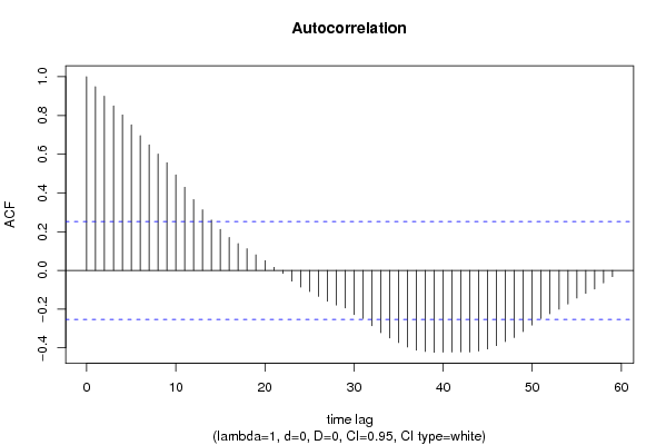
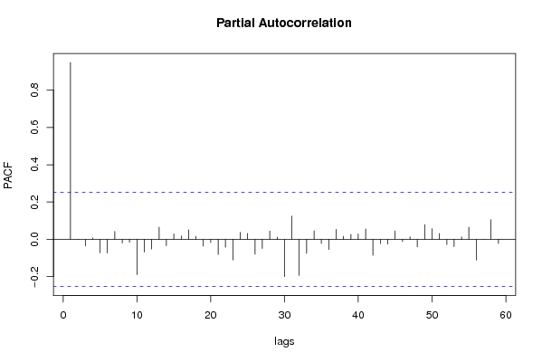
Title produced by software

(Partial) Autocorrelation Function

Date of computation

Thu, 26 Nov 2009 11:17:15 -0700

Cite this page as follows

Statistical Computations at FreeStatistics.org, Office for Research Development and Education, URL https://freestatistics.org/blog/index.php?v=date/2009/Nov/26/t1259259520yusf8b37w3mgqjs.htm/, Retrieved Mon, 29 Apr 2024 07:43:20 +0000

Statistical Computations at FreeStatistics.org, Office for Research Development and Education, URL https://freestatistics.org/blog/index.php?pk=60223, Retrieved Mon, 29 Apr 2024 07:43:20 +0000

QR Codes:

Paste this QR Code to cite your computation.

Original text written by user:

IsPrivate?

No (this computation is public)

User-defined keywords

Estimated Impact

126

Family? (F = Feedback message, R = changed R code, M = changed R Module, P = changed Parameters, D = changed Data)

-     [Univariate Explorative Data Analysis] [Run Sequence gebo...] [2008-12-12 13:32:37] [76963dc1903f0f612b6153510a3818cf]
- R  D  [Univariate Explorative Data Analysis] [Run Sequence gebo...] [2008-12-17 12:14:40] [76963dc1903f0f612b6153510a3818cf]
-         [Univariate Explorative Data Analysis] [Run Sequence Plot...] [2008-12-22 18:19:51] [1ce0d16c8f4225c977b42c8fa93bc163]
- RMP       [(Partial) Autocorrelation Function] [Identifying Integ...] [2009-11-22 12:16:10] [b98453cac15ba1066b407e146608df68]
-   PD          [(Partial) Autocorrelation Function] [cs.shw.ws8.v1.1] [2009-11-26 18:17:15] [47f146dd9fb230449e079c6cbc92f5f5] [Current]
-   P             [(Partial) Autocorrelation Function] [] [2009-11-30 16:53:41] [3af9fa3d2c04a43d660a9a466bdfbaa0] 

Feedback Forum

Post a new message

Dataseries X:

Download CSV

Histogram

Boxplots

Summary of computational transaction
Raw Input	view raw input (R code)
Raw Output	view raw output of R engine
Computing time	0 seconds
R Server	'Gwilym Jenkins' @ 72.249.127.135

\begin{tabular}{lllllllll}
\hline
Summary of computational transaction \tabularnewline
Raw Input & view raw input (R code)  \tabularnewline
Raw Output & view raw output of R engine  \tabularnewline
Computing time & 0 seconds \tabularnewline
R Server & 'Gwilym Jenkins' @ 72.249.127.135 \tabularnewline
\hline
\end{tabular}
%Source: https://freestatistics.org/blog/index.php?pk=60223&T=0

[TABLE]
[ROW][C]Summary of computational transaction[/C][/ROW]
[ROW][C]Raw Input[/C][C]view raw input (R code) [/C][/ROW]
[ROW][C]Raw Output[/C][C]view raw output of R engine [/C][/ROW]
[ROW][C]Computing time[/C][C]0 seconds[/C][/ROW]
[ROW][C]R Server[/C][C]'Gwilym Jenkins' @ 72.249.127.135[/C][/ROW]
[/TABLE]
Source: https://freestatistics.org/blog/index.php?pk=60223&T=0

Globally Unique Identifier (entire table): ba.freestatistics.org/blog/index.php?pk=60223&T=0

As an alternative you can also use a QR Code:

The GUIDs for individual cells are displayed in the table below:

Summary of computational transaction
Raw Input	view raw input (R code)
Raw Output	view raw output of R engine
Computing time	0 seconds
R Server	'Gwilym Jenkins' @ 72.249.127.135

Autocorrelation Function
Time lag k	ACF(k)	T-STAT	P-value
1	0.948314	7.3456	0
2	0.899238	6.9655	0
3	0.849246	6.5782	0
4	0.802748	6.2181	0
5	0.751448	5.8207	0
6	0.696023	5.3914	1e-06
7	0.648129	5.0204	2e-06
8	0.601098	4.6561	9e-06
9	0.55561	4.3037	3.1e-05
10	0.493302	3.8211	0.000159
11	0.429711	3.3285	0.000748
12	0.365865	2.834	0.003127
13	0.313461	2.4281	0.009098
14	0.259792	2.0123	0.02434
15	0.211642	1.6394	0.053185
16	0.170359	1.3196	0.095992
17	0.138604	1.0736	0.143645
18	0.112012	0.8676	0.194523
19	0.080676	0.6249	0.267198
20	0.050726	0.3929	0.347886
21	0.015687	0.1215	0.451847
22	-0.015959	-0.1236	0.451015
23	-0.055498	-0.4299	0.33441
24	-0.085718	-0.664	0.254627
25	-0.109086	-0.845	0.20074
26	-0.134241	-1.0398	0.151296
27	-0.159398	-1.2347	0.11088
28	-0.178818	-1.3851	0.085573
29	-0.194046	-1.5031	0.069032
30	-0.228503	-1.77	0.040906
31	-0.248336	-1.9236	0.029576
32	-0.285916	-2.2147	0.015295
33	-0.321192	-2.4879	0.007822
34	-0.348688	-2.7009	0.004487
35	-0.372481	-2.8852	0.002713
36	-0.395591	-3.0642	0.001634
37	-0.411769	-3.1895	0.001133
38	-0.418119	-3.2387	0.000979
39	-0.422504	-3.2727	0.000885
40	-0.422299	-3.2711	0.000889
41	-0.421297	-3.2634	0.00091
42	-0.420795	-3.2595	0.000921
43	-0.421319	-3.2635	0.000909
44	-0.416526	-3.2264	0.001016
45	-0.405231	-3.1389	0.001315
46	-0.388436	-3.0088	0.001915
47	-0.367192	-2.8443	0.00304
48	-0.346514	-2.6841	0.004694
49	-0.316102	-2.4485	0.008642
50	-0.282222	-2.1861	0.016361
51	-0.248101	-1.9218	0.029693
52	-0.223998	-1.7351	0.04393
53	-0.200068	-1.5497	0.063233
54	-0.173431	-1.3434	0.092103
55	-0.142957	-1.1073	0.136284
56	-0.118711	-0.9195	0.18075
57	-0.095933	-0.7431	0.230162
58	-0.06422	-0.4974	0.310346
59	-0.032473	-0.2515	0.401129
60	NA	NA	NA

\begin{tabular}{lllllllll}
\hline
Autocorrelation Function \tabularnewline
Time lag k & ACF(k) & T-STAT & P-value \tabularnewline
1 & 0.948314 & 7.3456 & 0 \tabularnewline
2 & 0.899238 & 6.9655 & 0 \tabularnewline
3 & 0.849246 & 6.5782 & 0 \tabularnewline
4 & 0.802748 & 6.2181 & 0 \tabularnewline
5 & 0.751448 & 5.8207 & 0 \tabularnewline
6 & 0.696023 & 5.3914 & 1e-06 \tabularnewline
7 & 0.648129 & 5.0204 & 2e-06 \tabularnewline
8 & 0.601098 & 4.6561 & 9e-06 \tabularnewline
9 & 0.55561 & 4.3037 & 3.1e-05 \tabularnewline
10 & 0.493302 & 3.8211 & 0.000159 \tabularnewline
11 & 0.429711 & 3.3285 & 0.000748 \tabularnewline
12 & 0.365865 & 2.834 & 0.003127 \tabularnewline
13 & 0.313461 & 2.4281 & 0.009098 \tabularnewline
14 & 0.259792 & 2.0123 & 0.02434 \tabularnewline
15 & 0.211642 & 1.6394 & 0.053185 \tabularnewline
16 & 0.170359 & 1.3196 & 0.095992 \tabularnewline
17 & 0.138604 & 1.0736 & 0.143645 \tabularnewline
18 & 0.112012 & 0.8676 & 0.194523 \tabularnewline
19 & 0.080676 & 0.6249 & 0.267198 \tabularnewline
20 & 0.050726 & 0.3929 & 0.347886 \tabularnewline
21 & 0.015687 & 0.1215 & 0.451847 \tabularnewline
22 & -0.015959 & -0.1236 & 0.451015 \tabularnewline
23 & -0.055498 & -0.4299 & 0.33441 \tabularnewline
24 & -0.085718 & -0.664 & 0.254627 \tabularnewline
25 & -0.109086 & -0.845 & 0.20074 \tabularnewline
26 & -0.134241 & -1.0398 & 0.151296 \tabularnewline
27 & -0.159398 & -1.2347 & 0.11088 \tabularnewline
28 & -0.178818 & -1.3851 & 0.085573 \tabularnewline
29 & -0.194046 & -1.5031 & 0.069032 \tabularnewline
30 & -0.228503 & -1.77 & 0.040906 \tabularnewline
31 & -0.248336 & -1.9236 & 0.029576 \tabularnewline
32 & -0.285916 & -2.2147 & 0.015295 \tabularnewline
33 & -0.321192 & -2.4879 & 0.007822 \tabularnewline
34 & -0.348688 & -2.7009 & 0.004487 \tabularnewline
35 & -0.372481 & -2.8852 & 0.002713 \tabularnewline
36 & -0.395591 & -3.0642 & 0.001634 \tabularnewline
37 & -0.411769 & -3.1895 & 0.001133 \tabularnewline
38 & -0.418119 & -3.2387 & 0.000979 \tabularnewline
39 & -0.422504 & -3.2727 & 0.000885 \tabularnewline
40 & -0.422299 & -3.2711 & 0.000889 \tabularnewline
41 & -0.421297 & -3.2634 & 0.00091 \tabularnewline
42 & -0.420795 & -3.2595 & 0.000921 \tabularnewline
43 & -0.421319 & -3.2635 & 0.000909 \tabularnewline
44 & -0.416526 & -3.2264 & 0.001016 \tabularnewline
45 & -0.405231 & -3.1389 & 0.001315 \tabularnewline
46 & -0.388436 & -3.0088 & 0.001915 \tabularnewline
47 & -0.367192 & -2.8443 & 0.00304 \tabularnewline
48 & -0.346514 & -2.6841 & 0.004694 \tabularnewline
49 & -0.316102 & -2.4485 & 0.008642 \tabularnewline
50 & -0.282222 & -2.1861 & 0.016361 \tabularnewline
51 & -0.248101 & -1.9218 & 0.029693 \tabularnewline
52 & -0.223998 & -1.7351 & 0.04393 \tabularnewline
53 & -0.200068 & -1.5497 & 0.063233 \tabularnewline
54 & -0.173431 & -1.3434 & 0.092103 \tabularnewline
55 & -0.142957 & -1.1073 & 0.136284 \tabularnewline
56 & -0.118711 & -0.9195 & 0.18075 \tabularnewline
57 & -0.095933 & -0.7431 & 0.230162 \tabularnewline
58 & -0.06422 & -0.4974 & 0.310346 \tabularnewline
59 & -0.032473 & -0.2515 & 0.401129 \tabularnewline
60 & NA & NA & NA \tabularnewline
\hline
\end{tabular}
%Source: https://freestatistics.org/blog/index.php?pk=60223&T=1

[TABLE]
[ROW][C]Autocorrelation Function[/C][/ROW]
[ROW][C]Time lag k[/C][C]ACF(k)[/C][C]T-STAT[/C][C]P-value[/C][/ROW]
[ROW][C]1[/C][C]0.948314[/C][C]7.3456[/C][C]0[/C][/ROW]
[ROW][C]2[/C][C]0.899238[/C][C]6.9655[/C][C]0[/C][/ROW]
[ROW][C]3[/C][C]0.849246[/C][C]6.5782[/C][C]0[/C][/ROW]
[ROW][C]4[/C][C]0.802748[/C][C]6.2181[/C][C]0[/C][/ROW]
[ROW][C]5[/C][C]0.751448[/C][C]5.8207[/C][C]0[/C][/ROW]
[ROW][C]6[/C][C]0.696023[/C][C]5.3914[/C][C]1e-06[/C][/ROW]
[ROW][C]7[/C][C]0.648129[/C][C]5.0204[/C][C]2e-06[/C][/ROW]
[ROW][C]8[/C][C]0.601098[/C][C]4.6561[/C][C]9e-06[/C][/ROW]
[ROW][C]9[/C][C]0.55561[/C][C]4.3037[/C][C]3.1e-05[/C][/ROW]
[ROW][C]10[/C][C]0.493302[/C][C]3.8211[/C][C]0.000159[/C][/ROW]
[ROW][C]11[/C][C]0.429711[/C][C]3.3285[/C][C]0.000748[/C][/ROW]
[ROW][C]12[/C][C]0.365865[/C][C]2.834[/C][C]0.003127[/C][/ROW]
[ROW][C]13[/C][C]0.313461[/C][C]2.4281[/C][C]0.009098[/C][/ROW]
[ROW][C]14[/C][C]0.259792[/C][C]2.0123[/C][C]0.02434[/C][/ROW]
[ROW][C]15[/C][C]0.211642[/C][C]1.6394[/C][C]0.053185[/C][/ROW]
[ROW][C]16[/C][C]0.170359[/C][C]1.3196[/C][C]0.095992[/C][/ROW]
[ROW][C]17[/C][C]0.138604[/C][C]1.0736[/C][C]0.143645[/C][/ROW]
[ROW][C]18[/C][C]0.112012[/C][C]0.8676[/C][C]0.194523[/C][/ROW]
[ROW][C]19[/C][C]0.080676[/C][C]0.6249[/C][C]0.267198[/C][/ROW]
[ROW][C]20[/C][C]0.050726[/C][C]0.3929[/C][C]0.347886[/C][/ROW]
[ROW][C]21[/C][C]0.015687[/C][C]0.1215[/C][C]0.451847[/C][/ROW]
[ROW][C]22[/C][C]-0.015959[/C][C]-0.1236[/C][C]0.451015[/C][/ROW]
[ROW][C]23[/C][C]-0.055498[/C][C]-0.4299[/C][C]0.33441[/C][/ROW]
[ROW][C]24[/C][C]-0.085718[/C][C]-0.664[/C][C]0.254627[/C][/ROW]
[ROW][C]25[/C][C]-0.109086[/C][C]-0.845[/C][C]0.20074[/C][/ROW]
[ROW][C]26[/C][C]-0.134241[/C][C]-1.0398[/C][C]0.151296[/C][/ROW]
[ROW][C]27[/C][C]-0.159398[/C][C]-1.2347[/C][C]0.11088[/C][/ROW]
[ROW][C]28[/C][C]-0.178818[/C][C]-1.3851[/C][C]0.085573[/C][/ROW]
[ROW][C]29[/C][C]-0.194046[/C][C]-1.5031[/C][C]0.069032[/C][/ROW]
[ROW][C]30[/C][C]-0.228503[/C][C]-1.77[/C][C]0.040906[/C][/ROW]
[ROW][C]31[/C][C]-0.248336[/C][C]-1.9236[/C][C]0.029576[/C][/ROW]
[ROW][C]32[/C][C]-0.285916[/C][C]-2.2147[/C][C]0.015295[/C][/ROW]
[ROW][C]33[/C][C]-0.321192[/C][C]-2.4879[/C][C]0.007822[/C][/ROW]
[ROW][C]34[/C][C]-0.348688[/C][C]-2.7009[/C][C]0.004487[/C][/ROW]
[ROW][C]35[/C][C]-0.372481[/C][C]-2.8852[/C][C]0.002713[/C][/ROW]
[ROW][C]36[/C][C]-0.395591[/C][C]-3.0642[/C][C]0.001634[/C][/ROW]
[ROW][C]37[/C][C]-0.411769[/C][C]-3.1895[/C][C]0.001133[/C][/ROW]
[ROW][C]38[/C][C]-0.418119[/C][C]-3.2387[/C][C]0.000979[/C][/ROW]
[ROW][C]39[/C][C]-0.422504[/C][C]-3.2727[/C][C]0.000885[/C][/ROW]
[ROW][C]40[/C][C]-0.422299[/C][C]-3.2711[/C][C]0.000889[/C][/ROW]
[ROW][C]41[/C][C]-0.421297[/C][C]-3.2634[/C][C]0.00091[/C][/ROW]
[ROW][C]42[/C][C]-0.420795[/C][C]-3.2595[/C][C]0.000921[/C][/ROW]
[ROW][C]43[/C][C]-0.421319[/C][C]-3.2635[/C][C]0.000909[/C][/ROW]
[ROW][C]44[/C][C]-0.416526[/C][C]-3.2264[/C][C]0.001016[/C][/ROW]
[ROW][C]45[/C][C]-0.405231[/C][C]-3.1389[/C][C]0.001315[/C][/ROW]
[ROW][C]46[/C][C]-0.388436[/C][C]-3.0088[/C][C]0.001915[/C][/ROW]
[ROW][C]47[/C][C]-0.367192[/C][C]-2.8443[/C][C]0.00304[/C][/ROW]
[ROW][C]48[/C][C]-0.346514[/C][C]-2.6841[/C][C]0.004694[/C][/ROW]
[ROW][C]49[/C][C]-0.316102[/C][C]-2.4485[/C][C]0.008642[/C][/ROW]
[ROW][C]50[/C][C]-0.282222[/C][C]-2.1861[/C][C]0.016361[/C][/ROW]
[ROW][C]51[/C][C]-0.248101[/C][C]-1.9218[/C][C]0.029693[/C][/ROW]
[ROW][C]52[/C][C]-0.223998[/C][C]-1.7351[/C][C]0.04393[/C][/ROW]
[ROW][C]53[/C][C]-0.200068[/C][C]-1.5497[/C][C]0.063233[/C][/ROW]
[ROW][C]54[/C][C]-0.173431[/C][C]-1.3434[/C][C]0.092103[/C][/ROW]
[ROW][C]55[/C][C]-0.142957[/C][C]-1.1073[/C][C]0.136284[/C][/ROW]
[ROW][C]56[/C][C]-0.118711[/C][C]-0.9195[/C][C]0.18075[/C][/ROW]
[ROW][C]57[/C][C]-0.095933[/C][C]-0.7431[/C][C]0.230162[/C][/ROW]
[ROW][C]58[/C][C]-0.06422[/C][C]-0.4974[/C][C]0.310346[/C][/ROW]
[ROW][C]59[/C][C]-0.032473[/C][C]-0.2515[/C][C]0.401129[/C][/ROW]
[ROW][C]60[/C][C]NA[/C][C]NA[/C][C]NA[/C][/ROW]
[/TABLE]
Source: https://freestatistics.org/blog/index.php?pk=60223&T=1

Globally Unique Identifier (entire table): ba.freestatistics.org/blog/index.php?pk=60223&T=1

As an alternative you can also use a QR Code:

The GUIDs for individual cells are displayed in the table below:

Autocorrelation Function
Time lag k	ACF(k)	T-STAT	P-value
1	0.948314	7.3456	0
2	0.899238	6.9655	0
3	0.849246	6.5782	0
4	0.802748	6.2181	0
5	0.751448	5.8207	0
6	0.696023	5.3914	1e-06
7	0.648129	5.0204	2e-06
8	0.601098	4.6561	9e-06
9	0.55561	4.3037	3.1e-05
10	0.493302	3.8211	0.000159
11	0.429711	3.3285	0.000748
12	0.365865	2.834	0.003127
13	0.313461	2.4281	0.009098
14	0.259792	2.0123	0.02434
15	0.211642	1.6394	0.053185
16	0.170359	1.3196	0.095992
17	0.138604	1.0736	0.143645
18	0.112012	0.8676	0.194523
19	0.080676	0.6249	0.267198
20	0.050726	0.3929	0.347886
21	0.015687	0.1215	0.451847
22	-0.015959	-0.1236	0.451015
23	-0.055498	-0.4299	0.33441
24	-0.085718	-0.664	0.254627
25	-0.109086	-0.845	0.20074
26	-0.134241	-1.0398	0.151296
27	-0.159398	-1.2347	0.11088
28	-0.178818	-1.3851	0.085573
29	-0.194046	-1.5031	0.069032
30	-0.228503	-1.77	0.040906
31	-0.248336	-1.9236	0.029576
32	-0.285916	-2.2147	0.015295
33	-0.321192	-2.4879	0.007822
34	-0.348688	-2.7009	0.004487
35	-0.372481	-2.8852	0.002713
36	-0.395591	-3.0642	0.001634
37	-0.411769	-3.1895	0.001133
38	-0.418119	-3.2387	0.000979
39	-0.422504	-3.2727	0.000885
40	-0.422299	-3.2711	0.000889
41	-0.421297	-3.2634	0.00091
42	-0.420795	-3.2595	0.000921
43	-0.421319	-3.2635	0.000909
44	-0.416526	-3.2264	0.001016
45	-0.405231	-3.1389	0.001315
46	-0.388436	-3.0088	0.001915
47	-0.367192	-2.8443	0.00304
48	-0.346514	-2.6841	0.004694
49	-0.316102	-2.4485	0.008642
50	-0.282222	-2.1861	0.016361
51	-0.248101	-1.9218	0.029693
52	-0.223998	-1.7351	0.04393
53	-0.200068	-1.5497	0.063233
54	-0.173431	-1.3434	0.092103
55	-0.142957	-1.1073	0.136284
56	-0.118711	-0.9195	0.18075
57	-0.095933	-0.7431	0.230162
58	-0.06422	-0.4974	0.310346
59	-0.032473	-0.2515	0.401129
60	NA	NA	NA

Partial Autocorrelation Function
Time lag k	PACF(k)	T-STAT	P-value
1	0.948314	7.3456	0
2	-0.000611	-0.0047	0.49812
3	-0.034316	-0.2658	0.395648
4	0.007289	0.0565	0.477582
5	-0.071882	-0.5568	0.28987
6	-0.07324	-0.5673	0.286309
7	0.04265	0.3304	0.371137
8	-0.019368	-0.15	0.440624
9	-0.01575	-0.122	0.451655
10	-0.189404	-1.4671	0.073783
11	-0.068228	-0.5285	0.299554
12	-0.052014	-0.4029	0.344227
13	0.065291	0.5057	0.307446
14	-0.033875	-0.2624	0.396957
15	0.02902	0.2248	0.411454
16	0.018677	0.1447	0.442727
17	0.051327	0.3976	0.346176
18	0.01668	0.1292	0.448816
19	-0.036457	-0.2824	0.389307
20	-0.017557	-0.136	0.446138
21	-0.08083	-0.6261	0.266809
22	-0.042164	-0.3266	0.372553
23	-0.110773	-0.858	0.197141
24	0.037645	0.2916	0.385799
25	0.031549	0.2444	0.403886
26	-0.079719	-0.6175	0.269621
27	-0.049053	-0.38	0.352659
28	0.044721	0.3464	0.365123
29	0.01178	0.0913	0.463799
30	-0.199786	-1.5475	0.063496
31	0.124756	0.9664	0.168873
32	-0.193657	-1.5001	0.069422
33	-0.075208	-0.5826	0.281185
34	0.045798	0.3547	0.362012
35	-0.021372	-0.1655	0.434536
36	-0.054504	-0.4222	0.3372
37	0.053571	0.415	0.339825
38	0.016486	0.1277	0.449406
39	0.026573	0.2058	0.418808
40	0.028489	0.2207	0.413046
41	0.055524	0.4301	0.334335
42	-0.085062	-0.6589	0.256244
43	-0.022828	-0.1768	0.43012
44	-0.025342	-0.1963	0.42252
45	0.045004	0.3486	0.364305
46	-0.011694	-0.0906	0.464063
47	0.013411	0.1039	0.458805
48	-0.040134	-0.3109	0.378485
49	0.07813	0.6052	0.273668
50	0.057451	0.445	0.328954
51	0.031472	0.2438	0.404117
52	-0.027561	-0.2135	0.415834
53	-0.039411	-0.3053	0.380605
54	0.013118	0.1016	0.459702
55	0.064927	0.5029	0.308429
56	-0.111605	-0.8645	0.195381
57	0.00022	0.0017	0.499324
58	0.104882	0.8124	0.209882
59	-0.022065	-0.1709	0.432432
60	NA	NA	NA

\begin{tabular}{lllllllll}
\hline
Partial Autocorrelation Function \tabularnewline
Time lag k & PACF(k) & T-STAT & P-value \tabularnewline
1 & 0.948314 & 7.3456 & 0 \tabularnewline
2 & -0.000611 & -0.0047 & 0.49812 \tabularnewline
3 & -0.034316 & -0.2658 & 0.395648 \tabularnewline
4 & 0.007289 & 0.0565 & 0.477582 \tabularnewline
5 & -0.071882 & -0.5568 & 0.28987 \tabularnewline
6 & -0.07324 & -0.5673 & 0.286309 \tabularnewline
7 & 0.04265 & 0.3304 & 0.371137 \tabularnewline
8 & -0.019368 & -0.15 & 0.440624 \tabularnewline
9 & -0.01575 & -0.122 & 0.451655 \tabularnewline
10 & -0.189404 & -1.4671 & 0.073783 \tabularnewline
11 & -0.068228 & -0.5285 & 0.299554 \tabularnewline
12 & -0.052014 & -0.4029 & 0.344227 \tabularnewline
13 & 0.065291 & 0.5057 & 0.307446 \tabularnewline
14 & -0.033875 & -0.2624 & 0.396957 \tabularnewline
15 & 0.02902 & 0.2248 & 0.411454 \tabularnewline
16 & 0.018677 & 0.1447 & 0.442727 \tabularnewline
17 & 0.051327 & 0.3976 & 0.346176 \tabularnewline
18 & 0.01668 & 0.1292 & 0.448816 \tabularnewline
19 & -0.036457 & -0.2824 & 0.389307 \tabularnewline
20 & -0.017557 & -0.136 & 0.446138 \tabularnewline
21 & -0.08083 & -0.6261 & 0.266809 \tabularnewline
22 & -0.042164 & -0.3266 & 0.372553 \tabularnewline
23 & -0.110773 & -0.858 & 0.197141 \tabularnewline
24 & 0.037645 & 0.2916 & 0.385799 \tabularnewline
25 & 0.031549 & 0.2444 & 0.403886 \tabularnewline
26 & -0.079719 & -0.6175 & 0.269621 \tabularnewline
27 & -0.049053 & -0.38 & 0.352659 \tabularnewline
28 & 0.044721 & 0.3464 & 0.365123 \tabularnewline
29 & 0.01178 & 0.0913 & 0.463799 \tabularnewline
30 & -0.199786 & -1.5475 & 0.063496 \tabularnewline
31 & 0.124756 & 0.9664 & 0.168873 \tabularnewline
32 & -0.193657 & -1.5001 & 0.069422 \tabularnewline
33 & -0.075208 & -0.5826 & 0.281185 \tabularnewline
34 & 0.045798 & 0.3547 & 0.362012 \tabularnewline
35 & -0.021372 & -0.1655 & 0.434536 \tabularnewline
36 & -0.054504 & -0.4222 & 0.3372 \tabularnewline
37 & 0.053571 & 0.415 & 0.339825 \tabularnewline
38 & 0.016486 & 0.1277 & 0.449406 \tabularnewline
39 & 0.026573 & 0.2058 & 0.418808 \tabularnewline
40 & 0.028489 & 0.2207 & 0.413046 \tabularnewline
41 & 0.055524 & 0.4301 & 0.334335 \tabularnewline
42 & -0.085062 & -0.6589 & 0.256244 \tabularnewline
43 & -0.022828 & -0.1768 & 0.43012 \tabularnewline
44 & -0.025342 & -0.1963 & 0.42252 \tabularnewline
45 & 0.045004 & 0.3486 & 0.364305 \tabularnewline
46 & -0.011694 & -0.0906 & 0.464063 \tabularnewline
47 & 0.013411 & 0.1039 & 0.458805 \tabularnewline
48 & -0.040134 & -0.3109 & 0.378485 \tabularnewline
49 & 0.07813 & 0.6052 & 0.273668 \tabularnewline
50 & 0.057451 & 0.445 & 0.328954 \tabularnewline
51 & 0.031472 & 0.2438 & 0.404117 \tabularnewline
52 & -0.027561 & -0.2135 & 0.415834 \tabularnewline
53 & -0.039411 & -0.3053 & 0.380605 \tabularnewline
54 & 0.013118 & 0.1016 & 0.459702 \tabularnewline
55 & 0.064927 & 0.5029 & 0.308429 \tabularnewline
56 & -0.111605 & -0.8645 & 0.195381 \tabularnewline
57 & 0.00022 & 0.0017 & 0.499324 \tabularnewline
58 & 0.104882 & 0.8124 & 0.209882 \tabularnewline
59 & -0.022065 & -0.1709 & 0.432432 \tabularnewline
60 & NA & NA & NA \tabularnewline
\hline
\end{tabular}
%Source: https://freestatistics.org/blog/index.php?pk=60223&T=2

[TABLE]
[ROW][C]Partial Autocorrelation Function[/C][/ROW]
[ROW][C]Time lag k[/C][C]PACF(k)[/C][C]T-STAT[/C][C]P-value[/C][/ROW]
[ROW][C]1[/C][C]0.948314[/C][C]7.3456[/C][C]0[/C][/ROW]
[ROW][C]2[/C][C]-0.000611[/C][C]-0.0047[/C][C]0.49812[/C][/ROW]
[ROW][C]3[/C][C]-0.034316[/C][C]-0.2658[/C][C]0.395648[/C][/ROW]
[ROW][C]4[/C][C]0.007289[/C][C]0.0565[/C][C]0.477582[/C][/ROW]
[ROW][C]5[/C][C]-0.071882[/C][C]-0.5568[/C][C]0.28987[/C][/ROW]
[ROW][C]6[/C][C]-0.07324[/C][C]-0.5673[/C][C]0.286309[/C][/ROW]
[ROW][C]7[/C][C]0.04265[/C][C]0.3304[/C][C]0.371137[/C][/ROW]
[ROW][C]8[/C][C]-0.019368[/C][C]-0.15[/C][C]0.440624[/C][/ROW]
[ROW][C]9[/C][C]-0.01575[/C][C]-0.122[/C][C]0.451655[/C][/ROW]
[ROW][C]10[/C][C]-0.189404[/C][C]-1.4671[/C][C]0.073783[/C][/ROW]
[ROW][C]11[/C][C]-0.068228[/C][C]-0.5285[/C][C]0.299554[/C][/ROW]
[ROW][C]12[/C][C]-0.052014[/C][C]-0.4029[/C][C]0.344227[/C][/ROW]
[ROW][C]13[/C][C]0.065291[/C][C]0.5057[/C][C]0.307446[/C][/ROW]
[ROW][C]14[/C][C]-0.033875[/C][C]-0.2624[/C][C]0.396957[/C][/ROW]
[ROW][C]15[/C][C]0.02902[/C][C]0.2248[/C][C]0.411454[/C][/ROW]
[ROW][C]16[/C][C]0.018677[/C][C]0.1447[/C][C]0.442727[/C][/ROW]
[ROW][C]17[/C][C]0.051327[/C][C]0.3976[/C][C]0.346176[/C][/ROW]
[ROW][C]18[/C][C]0.01668[/C][C]0.1292[/C][C]0.448816[/C][/ROW]
[ROW][C]19[/C][C]-0.036457[/C][C]-0.2824[/C][C]0.389307[/C][/ROW]
[ROW][C]20[/C][C]-0.017557[/C][C]-0.136[/C][C]0.446138[/C][/ROW]
[ROW][C]21[/C][C]-0.08083[/C][C]-0.6261[/C][C]0.266809[/C][/ROW]
[ROW][C]22[/C][C]-0.042164[/C][C]-0.3266[/C][C]0.372553[/C][/ROW]
[ROW][C]23[/C][C]-0.110773[/C][C]-0.858[/C][C]0.197141[/C][/ROW]
[ROW][C]24[/C][C]0.037645[/C][C]0.2916[/C][C]0.385799[/C][/ROW]
[ROW][C]25[/C][C]0.031549[/C][C]0.2444[/C][C]0.403886[/C][/ROW]
[ROW][C]26[/C][C]-0.079719[/C][C]-0.6175[/C][C]0.269621[/C][/ROW]
[ROW][C]27[/C][C]-0.049053[/C][C]-0.38[/C][C]0.352659[/C][/ROW]
[ROW][C]28[/C][C]0.044721[/C][C]0.3464[/C][C]0.365123[/C][/ROW]
[ROW][C]29[/C][C]0.01178[/C][C]0.0913[/C][C]0.463799[/C][/ROW]
[ROW][C]30[/C][C]-0.199786[/C][C]-1.5475[/C][C]0.063496[/C][/ROW]
[ROW][C]31[/C][C]0.124756[/C][C]0.9664[/C][C]0.168873[/C][/ROW]
[ROW][C]32[/C][C]-0.193657[/C][C]-1.5001[/C][C]0.069422[/C][/ROW]
[ROW][C]33[/C][C]-0.075208[/C][C]-0.5826[/C][C]0.281185[/C][/ROW]
[ROW][C]34[/C][C]0.045798[/C][C]0.3547[/C][C]0.362012[/C][/ROW]
[ROW][C]35[/C][C]-0.021372[/C][C]-0.1655[/C][C]0.434536[/C][/ROW]
[ROW][C]36[/C][C]-0.054504[/C][C]-0.4222[/C][C]0.3372[/C][/ROW]
[ROW][C]37[/C][C]0.053571[/C][C]0.415[/C][C]0.339825[/C][/ROW]
[ROW][C]38[/C][C]0.016486[/C][C]0.1277[/C][C]0.449406[/C][/ROW]
[ROW][C]39[/C][C]0.026573[/C][C]0.2058[/C][C]0.418808[/C][/ROW]
[ROW][C]40[/C][C]0.028489[/C][C]0.2207[/C][C]0.413046[/C][/ROW]
[ROW][C]41[/C][C]0.055524[/C][C]0.4301[/C][C]0.334335[/C][/ROW]
[ROW][C]42[/C][C]-0.085062[/C][C]-0.6589[/C][C]0.256244[/C][/ROW]
[ROW][C]43[/C][C]-0.022828[/C][C]-0.1768[/C][C]0.43012[/C][/ROW]
[ROW][C]44[/C][C]-0.025342[/C][C]-0.1963[/C][C]0.42252[/C][/ROW]
[ROW][C]45[/C][C]0.045004[/C][C]0.3486[/C][C]0.364305[/C][/ROW]
[ROW][C]46[/C][C]-0.011694[/C][C]-0.0906[/C][C]0.464063[/C][/ROW]
[ROW][C]47[/C][C]0.013411[/C][C]0.1039[/C][C]0.458805[/C][/ROW]
[ROW][C]48[/C][C]-0.040134[/C][C]-0.3109[/C][C]0.378485[/C][/ROW]
[ROW][C]49[/C][C]0.07813[/C][C]0.6052[/C][C]0.273668[/C][/ROW]
[ROW][C]50[/C][C]0.057451[/C][C]0.445[/C][C]0.328954[/C][/ROW]
[ROW][C]51[/C][C]0.031472[/C][C]0.2438[/C][C]0.404117[/C][/ROW]
[ROW][C]52[/C][C]-0.027561[/C][C]-0.2135[/C][C]0.415834[/C][/ROW]
[ROW][C]53[/C][C]-0.039411[/C][C]-0.3053[/C][C]0.380605[/C][/ROW]
[ROW][C]54[/C][C]0.013118[/C][C]0.1016[/C][C]0.459702[/C][/ROW]
[ROW][C]55[/C][C]0.064927[/C][C]0.5029[/C][C]0.308429[/C][/ROW]
[ROW][C]56[/C][C]-0.111605[/C][C]-0.8645[/C][C]0.195381[/C][/ROW]
[ROW][C]57[/C][C]0.00022[/C][C]0.0017[/C][C]0.499324[/C][/ROW]
[ROW][C]58[/C][C]0.104882[/C][C]0.8124[/C][C]0.209882[/C][/ROW]
[ROW][C]59[/C][C]-0.022065[/C][C]-0.1709[/C][C]0.432432[/C][/ROW]
[ROW][C]60[/C][C]NA[/C][C]NA[/C][C]NA[/C][/ROW]
[/TABLE]
Source: https://freestatistics.org/blog/index.php?pk=60223&T=2

Globally Unique Identifier (entire table): ba.freestatistics.org/blog/index.php?pk=60223&T=2

As an alternative you can also use a QR Code:

The GUIDs for individual cells are displayed in the table below:

Partial Autocorrelation Function
Time lag k	PACF(k)	T-STAT	P-value
1	0.948314	7.3456	0
2	-0.000611	-0.0047	0.49812
3	-0.034316	-0.2658	0.395648
4	0.007289	0.0565	0.477582
5	-0.071882	-0.5568	0.28987
6	-0.07324	-0.5673	0.286309
7	0.04265	0.3304	0.371137
8	-0.019368	-0.15	0.440624
9	-0.01575	-0.122	0.451655
10	-0.189404	-1.4671	0.073783
11	-0.068228	-0.5285	0.299554
12	-0.052014	-0.4029	0.344227
13	0.065291	0.5057	0.307446
14	-0.033875	-0.2624	0.396957
15	0.02902	0.2248	0.411454
16	0.018677	0.1447	0.442727
17	0.051327	0.3976	0.346176
18	0.01668	0.1292	0.448816
19	-0.036457	-0.2824	0.389307
20	-0.017557	-0.136	0.446138
21	-0.08083	-0.6261	0.266809
22	-0.042164	-0.3266	0.372553
23	-0.110773	-0.858	0.197141
24	0.037645	0.2916	0.385799
25	0.031549	0.2444	0.403886
26	-0.079719	-0.6175	0.269621
27	-0.049053	-0.38	0.352659
28	0.044721	0.3464	0.365123
29	0.01178	0.0913	0.463799
30	-0.199786	-1.5475	0.063496
31	0.124756	0.9664	0.168873
32	-0.193657	-1.5001	0.069422
33	-0.075208	-0.5826	0.281185
34	0.045798	0.3547	0.362012
35	-0.021372	-0.1655	0.434536
36	-0.054504	-0.4222	0.3372
37	0.053571	0.415	0.339825
38	0.016486	0.1277	0.449406
39	0.026573	0.2058	0.418808
40	0.028489	0.2207	0.413046
41	0.055524	0.4301	0.334335
42	-0.085062	-0.6589	0.256244
43	-0.022828	-0.1768	0.43012
44	-0.025342	-0.1963	0.42252
45	0.045004	0.3486	0.364305
46	-0.011694	-0.0906	0.464063
47	0.013411	0.1039	0.458805
48	-0.040134	-0.3109	0.378485
49	0.07813	0.6052	0.273668
50	0.057451	0.445	0.328954
51	0.031472	0.2438	0.404117
52	-0.027561	-0.2135	0.415834
53	-0.039411	-0.3053	0.380605
54	0.013118	0.1016	0.459702
55	0.064927	0.5029	0.308429
56	-0.111605	-0.8645	0.195381
57	0.00022	0.0017	0.499324
58	0.104882	0.8124	0.209882
59	-0.022065	-0.1709	0.432432
60	NA	NA	NA

Figure 1

PNG link

Postscript link

PDF link

Figure 2

PNG link

Postscript link

PDF link

Parameters (Session):

par1 = 60 ; par2 = 1 ; par3 = 0 ; par4 = 0 ; par5 = 12 ; par6 = White Noise ; par7 = 0.95 ;

Parameters (R input):

par1 = 60 ; par2 = 1 ; par3 = 0 ; par4 = 0 ; par5 = 12 ; par6 = White Noise ; par7 = 0.95 ;

R code (references can be found in the software module):

if (par1 == 'Default') {
par1 = 10*log10(length(x))
} else {
par1 <- as.numeric(par1)
}
par2 <- as.numeric(par2)
par3 <- as.numeric(par3)
par4 <- as.numeric(par4)
par5 <- as.numeric(par5)
if (par6 == 'White Noise') par6 <- 'white' else par6 <- 'ma'
par7 <- as.numeric(par7)
if (par2 == 0) {
x <- log(x)
} else {
x <- (x ^ par2 - 1) / par2
}
if (par3 > 0) x <- diff(x,lag=1,difference=par3)
if (par4 > 0) x <- diff(x,lag=par5,difference=par4)
bitmap(file='pic1.png')
racf <- acf(x, par1, main='Autocorrelation', xlab='time lag', ylab='ACF', ci.type=par6, ci=par7, sub=paste('(lambda=',par2,', d=',par3,', D=',par4,', CI=', par7, ', CI type=',par6,')',sep=''))
dev.off()
bitmap(file='pic2.png')
rpacf <- pacf(x,par1,main='Partial Autocorrelation',xlab='lags',ylab='PACF')
dev.off()
(myacf <- c(racf$acf))
(mypacf <- c(rpacf$acf))
lengthx <- length(x)
sqrtn <- sqrt(lengthx)
load(file='createtable')
a<-table.start()
a<-table.row.start(a)
a<-table.element(a,'Autocorrelation Function',4,TRUE)
a<-table.row.end(a)
a<-table.row.start(a)
a<-table.element(a,'Time lag k',header=TRUE)
a<-table.element(a,hyperlink('basics.htm','ACF(k)','click here for more information about the Autocorrelation Function'),header=TRUE)
a<-table.element(a,'T-STAT',header=TRUE)
a<-table.element(a,'P-value',header=TRUE)
a<-table.row.end(a)
for (i in 2:(par1+1)) {
a<-table.row.start(a)
a<-table.element(a,i-1,header=TRUE)
a<-table.element(a,round(myacf[i],6))
mytstat <- myacf[i]*sqrtn
a<-table.element(a,round(mytstat,4))
a<-table.element(a,round(1-pt(abs(mytstat),lengthx),6))
a<-table.row.end(a)
}
a<-table.end(a)
table.save(a,file='mytable.tab')
a<-table.start()
a<-table.row.start(a)
a<-table.element(a,'Partial Autocorrelation Function',4,TRUE)
a<-table.row.end(a)
a<-table.row.start(a)
a<-table.element(a,'Time lag k',header=TRUE)
a<-table.element(a,hyperlink('basics.htm','PACF(k)','click here for more information about the Partial Autocorrelation Function'),header=TRUE)
a<-table.element(a,'T-STAT',header=TRUE)
a<-table.element(a,'P-value',header=TRUE)
a<-table.row.end(a)
for (i in 1:par1) {
a<-table.row.start(a)
a<-table.element(a,i,header=TRUE)
a<-table.element(a,round(mypacf[i],6))
mytstat <- mypacf[i]*sqrtn
a<-table.element(a,round(mytstat,4))
a<-table.element(a,round(1-pt(abs(mytstat),lengthx),6))
a<-table.row.end(a)
}
a<-table.end(a)
table.save(a,file='mytable1.tab')

Free Statistics

Description of Statistical Computation

Tree of Dependent Computations

Dataset

Tables (Output of Computation)

Figures (Output of Computation)

Input Parameters & R Code